BCA 3RD SEM OS NOTES 2023-24
UNIT 1
Time Sharing Operating System
Multiprogrammed, batched systems provided an environment where various system resources were used effectively, but it did not provide for user interaction with computer systems. Time sharing is a logical extension of multiprogramming. The CPU performs many tasks by switches are so frequent that the user can interact with each program while it is running.
A time shared operating system allows multiple users to share computers simultaneously. Each action or order at a time the shared system becomes smaller, so only a little CPU time is required for each user. As the system rapidly switches from one user to another, each user is given the impression that the entire computer system is dedicated to its use, although it is being shared among multiple users.
Attention reader! Don’t stop learning now. Get hold of all the important CS Theory concepts for SDE interviews with the CS Theory Course at a student-friendly price and become industry ready.
A time shared operating system uses CPU scheduling and multi-programming to provide each with a small portion of a shared computer at once. Each user has at least one separate program in memory. A program loaded into memory and executes, it performs a short period of time either before completion or to complete I/O.This short period of time during which user gets attention of CPU is known as time slice, time slot or quantum.It is typically of the order of 10 to 100 milliseconds. Time shared operating systems are more complex than multiprogrammed operating systems. In both, multiple jobs must be kept in memory simultaneously, so the system must have memory management and security. To achieve a good response time, jobs may have to swap in and out of disk from main memory which now serves as a backing store for main memory. A common method to achieve this goal is virtual memory, a technique that allows the execution of a job that may not be completely in memory.
In above figure the user 5 is active state but user 1, user 2, user 3, and user 4 are in waiting state whereas user 6 is in ready state.
1. Active State –
The user’s program is under the control of CPU. Only one program is available in this state.
2. Ready State –
The user program is ready to execute but it is waiting for for it’s turn to get the CPU.More than one user can be in ready state at a time.
3. Waiting State –
The user’s program is waiting for some input/output operation. More than one user can be in a waiting state at a time.
Requirements of Time Sharing Operating System :
An alarm clock mechanism to send an interrupt signal to the CPU after every time slice. Memory Protection mechanism to prevent one job’s instructions and data from interfering with other jobs.
Advantages :
1. Each task gets an equal opportunity.
2. Less chances of duplication of software.
3. CPU idle time can be reduced.
Disadvantages :
1. Reliability problem.
2. One must have to take of security and integrity of user programs and data.
3. Data communication problem.
What is Parallel Processing ?
For the purpose of increasing the computational speed of computer system, the term ‘parallel processing‘ employed to give simultaneous data-processing operations is used to represent a large class. In addition, a parallel processing system is capable of concurrent data processing to achieve faster execution times.
As an example, the next instruction can be read from memory, while an instruction is being executed in ALU. The system can have two or more ALUs and be able to execute two or more instructions at the same time. In addition, two or more processing is also used to speed up computer processing capacity and increases with parallel processing, and with it, the cost of the system increases. But, technological development has reduced hardware costs to the point where parallel processing methods are economically possible.
Attention reader! Don’t stop learning now. Get hold of all the important CS Theory concepts for SDE interviews with the CS Theory Course at a student-friendly price and become industry ready.
Parallel processing derives from multiple levels of complexity. It is distinguished between parallel and serial operations by the type of registers used at the lowest level. Shift registers work one bit at a time in a serial fashion, while parallel registers work simultaneously with all bits of simultaneously with all bits of the word. At high levels of complexity, parallel processing derives from having a plurality of functional units that perform separate or similar operations simultaneously. By distributing data among several functional units, parallel processing is installed.
Types of Operating Systems
An Operating System performs all the basic tasks like managing files, processes, and memory. Thus operating system acts as the manager of all the resources, i.e. resource manager. Thus, the operating system becomes an interface between user and machine.
Types of Operating Systems: Some widely used operating systems are as follows-
Attention reader! All those who say programming isn't for kids, just haven't met the right mentors yet. Join the Demo Class for First Step to Coding Course, specifically designed for students of class 8 to 12.
The students will get to learn more about the world of programming in these free classes which will definitely help them in making a wise career choice in the future.
1. Batch Operating System –
This type of operating system does not interact with the computer directly. There is an operator which takes similar jobs having the same requirement and group them into batches. It is the responsibility of the operator to sort jobs with similar needs.
Advantages of Batch Operating System:
· It is very difficult to guess or know the time required for any job to complete. Processors of the batch systems know how long the job would be when it is in queue
· Multiple users can share the batch systems
· The idle time for the batch system is very less
· It is easy to manage large work repeatedly in batch systems
Disadvantages of Batch Operating System:
· The computer operators should be well known with batch systems
· Batch systems are hard to debug
· It is sometimes costly
· The other jobs will have to wait for an unknown time if any job fails
Examples of Batch based Operating System: Payroll System, Bank Statements, etc.
2. Time-Sharing Operating Systems –
Each task is given some time to execute so that all the tasks work smoothly. Each user gets the time of CPU as they use a single system. These systems are also known as Multitasking Systems. The task can be from a single user or different users also. The time that each task gets to execute is called quantum. After this time interval is over OS switches over to the next task.
Advantages of Time-Sharing OS:
· Each task gets an equal opportunity
· Fewer chances of duplication of software
· CPU idle time can be reduced
Disadvantages of Time-Sharing OS:
· Reliability problem
· One must have to take care of the security and integrity of user programs and data
· Data communication problem
Examples of Time-Sharing OSs are: Multics, Unix, etc.
3. Distributed Operating System –
These types of the operating system is a recent advancement in the world of computer technology and are being widely accepted all over the world and, that too, with a great pace. Various autonomous interconnected computers communicate with each other using a shared communication network. Independent systems possess their own memory unit and CPU. These are referred to as loosely coupled systems or distributed systems. These system’s processors differ in size and function. The major benefit of working with these types of the operating system is that it is always possible that one user can access the files or software which are not actually present on his system but some other system connected within this network i.e., remote access is enabled within the devices connected in that network.
Advantages of Distributed Operating System:
· Failure of one will not affect the other network communication, as all systems are independent from each other
· Electronic mail increases the data exchange speed
· Since resources are being shared, computation is highly fast and durable
· Load on host computer reduces
· These systems are easily scalable as many systems can be easily added to the network
· Delay in data processing reduces
Disadvantages of Distributed Operating System:
· Failure of the main network will stop the entire communication
· To establish distributed systems the language which is used are not well defined yet
· These types of systems are not readily available as they are very expensive. Not only that the underlying software is highly complex and not understood well yet
Examples of Distributed Operating System are- LOCUS, etc.
4. Network Operating System –
These systems run on a server and provide the capability to manage data, users, groups, security, applications, and other networking functions. These types of operating systems allow shared access of files, printers, security, applications, and other networking functions over a small private network. One more important aspect of Network Operating Systems is that all the users are well aware of the underlying configuration, of all other users within the network, their individual connections, etc. and that’s why these computers are popularly known as tightly coupled systems.
Advantages of Network Operating System:
· Highly stable centralized servers
· Security concerns are handled through servers
· New technologies and hardware up-gradation are easily integrated into the system
· Server access is possible remotely from different locations and types of systems
Disadvantages of Network Operating System:
· Servers are costly
· User has to depend on a central location for most operations
· Maintenance and updates are required regularly
Examples of Network Operating System are: Microsoft Windows Server 2003, Microsoft Windows Server 2008, UNIX, Linux, Mac OS X, Novell NetWare, and BSD, etc.
5. Real-Time Operating System –
These types of OSs serve real-time systems. The time interval required to process and respond to inputs is very small. This time interval is called response time.
Real-time systems are used when there are time requirements that are very strict like missile systems, air traffic control systems, robots, etc.
Two types of Real-Time Operating System which are as follows:
· Hard Real-Time Systems:
These OSs are meant for applications where time constraints are very strict and even the shortest possible delay is not acceptable. These systems are built for saving life like automatic parachutes or airbags which are required to be readily available in case of any accident. Virtual memory is rarely found in these systems.
· Soft Real-Time Systems:
These OSs are for applications where for time-constraint is less strict.
Advantages of RTOS:
· Maximum Consumption: Maximum utilization of devices and system, thus more output from all the resources
· Task Shifting: The time assigned for shifting tasks in these systems are very less. For example, in older systems, it takes about 10 microseconds in shifting one task to another, and in the latest systems, it takes 3 microseconds.
· Focus on Application: Focus on running applications and less importance to applications which are in the queue.
· Real-time operating system in the embedded system: Since the size of programs are small, RTOS can also be used in embedded systems like in transport and others.
· Error Free: These types of systems are error-free.
· Memory Allocation: Memory allocation is best managed in these types of systems.
Disadvantages of RTOS:
· Limited Tasks: Very few tasks run at the same time and their concentration is very less on few applications to avoid errors.
· Use heavy system resources: Sometimes the system resources are not so good and they are expensive as well.
· Complex Algorithms: The algorithms are very complex and difficult for the designer to write on.
· Device driver and interrupt signals: It needs specific device drivers and interrupts signals to respond earliest to interrupts.
· Thread Priority: It is not good to set thread priority as these systems are very less prone to switching tasks.
Examples of Real-Time Operating Systems are: Scientific experiments, medical imaging systems, industrial control systems, weapon systems, robots, air traffic control systems, etc.
.
Memory Organisation in Computer Architecture
The memory is organized in the form of a cell, each cell is able to be identified with a unique number called address. Each cell is able to recognize control signals such as “read” and “write”, generated by CPU when it wants to read or write address. Whenever CPU executes the program there is a need to transfer the instruction from the memory to CPU because the program is available in memory. To access the instruction CPU generates the memory request
Memory Management in Operating System
The term Memory can be defined as a collection of data in a specific format. It is used to store instructions and processed data. The memory comprises a large array or group of words or bytes, each with its own location. The primary motive of a computer system is to execute programs. These programs, along with the information they access, should be in the main memory during execution. The CPU fetches instructions from memory according to the value of the program counter.
To achieve a degree of multiprogramming and proper utilization of memory, memory management is important. Many memory management methods exist, reflecting various approaches, and the effectiveness of each algorithm depends on the situation.
What is Main Memory:
The main memory is central to the operation of a modern computer. Main Memory is a large array of words or bytes, ranging in size from hundreds of thousands to billions. Main memory is a repository of rapidly available information shared by the CPU and I/O devices. Main memory is the place where programs and information are kept when the processor is effectively utilizing them. Main memory is associated with the processor, so moving instructions and information into and out of the processor is extremely fast. Main memory is also known as RAM(Random Access Memory). This memory is a volatile memory.RAM lost its data when a power interruption occurs.

Figure 1: Memory hierarchy
What is Memory Management :
In a multiprogramming computer, the operating system resides in a part of memory and the rest is used by multiple processes. The task of subdividing the memory among different processes is called memory management. Memory management is a method in the operating system to manage operations between main memory and disk during process execution. The main aim of memory management is to achieve efficient utilization of memory.
Why Memory Management is required:
Allocate and de-allocate memory before and after process execution.
To keep track of used memory space by processes.
To minimize fragmentation issues.
To proper utilization of main memory.
To maintain data integrity while executing of process.
Now we are discussing the concept of logical address space and Physical address space:
Logical and Physical Address Space:
Logical Address space: An address generated by the CPU is known as “Logical Address”. It is also known as a Virtual address. Logical address space can be defined as the size of the process. A logical address can be changed.
Physical Address space: An address seen by the memory unit (i.e the one loaded into the memory address register of the memory) is commonly known as a “Physical Address”. A Physical address is also known as a Real address. The set of all physical addresses corresponding to these logical addresses is known as Physical address space. A physical address is computed by MMU. The run-time mapping from virtual to physical addresses is done by a hardware device Memory Management Unit(MMU). The physical address always remains constant.
Static and Dynamic Loading:
To load a process into the main memory is done by a loader. There are two different types of loading :
Static loading:- loading the entire program into a fixed address. It requires more memory space.
Dynamic loading:- The entire program and all data of a process must be in physical memory for the process to execute. So, the size of a process is limited to the size of physical memory. To gain proper memory utilization, dynamic loading is used. In dynamic loading, a routine is not loaded until it is called. All routines are residing on disk in a relocatable load format. One of the advantages of dynamic loading is that unused routine is never loaded. This loading is useful when a large amount of code is needed to handle it efficiently.
Static and Dynamic linking:
To perform a linking task a linker is used. A linker is a program that takes one or more object files generated by a compiler and combines them into a single executable file.
Static linking: In static linking, the linker combines all necessary program modules into a single executable program. So there is no runtime dependency. Some operating systems support only static linking, in which system language libraries are treated like any other object module.
Dynamic linking: The basic concept of dynamic linking is similar to dynamic loading. In dynamic linking, “Stub” is included for each appropriate library routine reference. A stub is a small piece of code. When the stub is executed, it checks whether the needed routine is already in memory or not. If not available then the program loads the routine into memory.
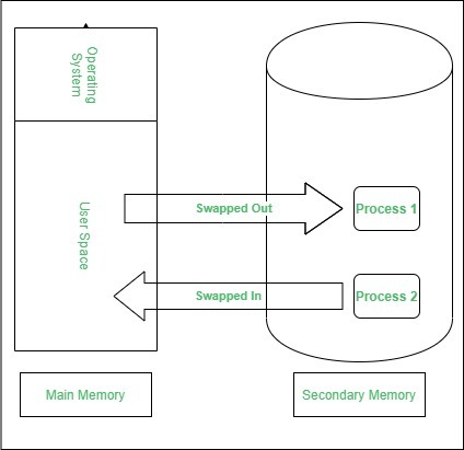
Swapping :
When a process is executed it must have resided in memory. Swapping is a process of swap a process temporarily into a secondary memory from the main memory, which is fast as compared to secondary memory. A swapping allows more processes to be run and can be fit into memory at one time. The main part of swapping is transferred time and the total time directly proportional to the amount of memory swapped. Swapping is also known as roll-out, roll in, because if a higher priority process arrives and wants service, the memory manager can swap out the lower priority process and then load and execute the higher priority process. After finishing higher priority work, the lower priority process swapped back in memory and continued to the execution process.
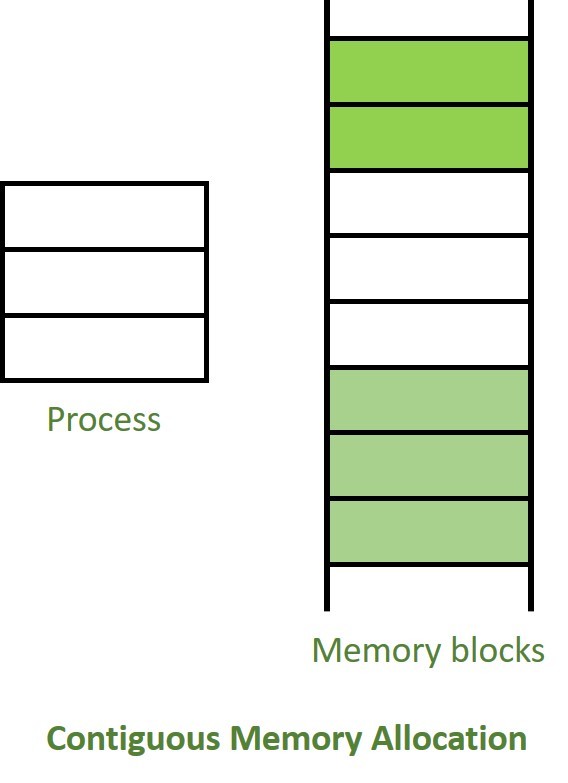
Contiguous Memory Allocation :
The main memory should oblige both the operating system and the different client processes. Therefore, the allocation of memory becomes an important task in the operating system. The memory is usually divided into two partitions: one for the resident operating system and one for the user processes. We normally need several user processes to reside in memory simultaneously. Therefore, we need to consider how to allocate available memory to the processes that are in the input queue waiting to be brought into memory. In adjacent memory allotment, each process is contained in a single contiguous segment of memory.
Memory allocation:
To gain proper memory utilization, memory allocation must be allocated efficient manner. One of the simplest methods for allocating memory is to divide memory into several fixed-sized partitions and each partition contains exactly one process. Thus, the degree of multiprogramming is obtained by the number of partitions.
Multiple partition allocation: In this method, a process is selected from the input queue and loaded into the free partition. When the process terminates, the partition becomes available for other processes.
Fixed partition allocation: In this method, the operating system maintains a table that indicates which parts of memory are available and which are occupied by processes. Initially, all memory is available for user processes and is considered one large block of available memory. This available memory is known as “Hole”. When the process arrives and needs memory, we search for a hole that is large enough to store this process. If the requirement fulfills then we allocate memory to process, otherwise keeping the rest available to satisfy future requests. While allocating a memory sometimes dynamic storage allocation problems occur, which concerns how to satisfy a request of size n from a list of free holes. There are some solutions to this problem:
First fit:-
In the first fit, the first available free hole fulfills the requirement of the process allocated.
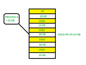
Here, in this diagram 40 KB memory block is the first available free hole that can store process A (size of 25 KB), because the first two blocks did not have sufficient memory space.
Best fit:-
In the best fit, allocate the smallest hole that is big enough to process requirements. For this, we search the entire list, unless the list is ordered by size.
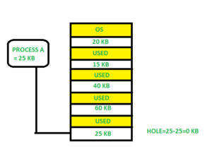
Here in this example, first, we traverse the complete list and find the last hole 25KB is the best suitable hole for Process A(size 25KB).
In this method memory utilization is maximum as compared to other memory allocation techniques.
Worst fit:-In the worst fit, allocate the largest available hole to process. This method produces the largest leftover hole.
Here in this example, Process A (Size 25 KB) is allocated to the largest available memory block which is 60KB. Inefficient memory utilization is a major issue in the worst fit.
Fragmentation:
A Fragmentation is defined as when the process is loaded and removed after execution from memory, it creates a small free hole. These holes can not be assigned to new processes because holes are not combined or do not fulfill the memory requirement of the process. To achieve a degree of multiprogramming, we must reduce the waste of memory or fragmentation problem. In operating system two types of fragmentation:
Internal fragmentation:
Internal fragmentation occurs when memory blocks are allocated to the process more than their requested size. Due to this some unused space is leftover and creates an internal fragmentation problem.
Example: Suppose there is a fixed partitioning is used for memory allocation and the different size of block 3MB, 6MB, and 7MB space in memory. Now a new process p4 of size 2MB comes and demand for the block of memory. It gets a memory block of 3MB but 1MB block memory is a waste, and it can not be allocated to other processes too. This is called internal fragmentation.
External fragmentation:
In external fragmentation, we have a free memory block, but we can not assign it to process because blocks are not contiguous.
Example: Suppose (consider above example) three process p1, p2, p3 comes with size 2MB, 4MB, and 7MB respectively. Now they get memory blocks of size 3MB, 6MB, and 7MB allocated respectively. After allocating process p1 process and p2 process left 1MB and 2MB. Suppose a new process p4 comes and demands a 3MB block of memory, which is available, but we can not assign it because free memory space is not contiguous. This is called external fragmentation.
Both the first fit and best-fit systems for memory allocation affected by external fragmentation. To overcome the external fragmentation problem Compaction is used. In the compaction technique, all free memory space combines and makes one large block. So, this space can be used by other processes effectively.
Another possible solution to the external fragmentation is to allow the logical address space of the processes to be noncontiguous, thus permit a process to be allocated physical memory where ever the latter is available.
Paging:
Paging is a memory management scheme that eliminates the need for contiguous allocation of physical memory. This scheme permits the physical address space of a process to be non-contiguous.
Logical Address or Virtual Address (represented in bits): An address generated by the CPU
Logical Address Space or Virtual Address Space (represented in words or bytes): The set of all logical addresses generated by a program
Physical Address (represented in bits): An address actually available on a memory unit
Physical Address Space (represented in words or bytes): The set of all physical addresses corresponding to the logical addresses
Example:
If Logical Address = 31 bits, then Logical Address Space = 231 words = 2 G words (1 G = 230)
If Logical Address Space = 128 M words = 27 * 220 words, then Logical Address = log2 227 = 27 bits
If Physical Address = 22 bits, then Physical Address Space = 222 words = 4 M words (1 M = 220)
If Physical Address Space = 16 M words = 24 * 220 words, then Physical Address = log2 224 = 24 bits
The mapping from virtual to physical address is done by the memory management unit (MMU) which is a hardware device and this mapping is known as the paging technique.
The Physical Address Space is conceptually divided into several fixed-size blocks, called frames.
The Logical Address Space is also split into fixed-size blocks, called pages.
Page Size = Frame Size
Let us consider an example:
Physical Address = 12 bits, then Physical Address Space = 4 K words
Logical Address = 13 bits, then Logical Address Space = 8 K words
Page size = frame size = 1 K words (assumption)
The address generated by the CPU is divided into
Page number(p): Number of bits required to represent the pages in Logical Address Space or Page number
Page offset(d): Number of bits required to represent a particular word in a page or page size of Logical Address Space or word number of a page or page offset.
Physical Address is divided into
Frame number(f): Number of bits required to represent the frame of Physical Address Space or Frame number frame
Frame offset(d): Number of bits required to represent a particular word in a frame or frame size of Physical Address Space or word number of a frame or frame offset.
The hardware implementation of the page table can be done by using dedicated registers. But the usage of register for the page table is satisfactory only if the page table is small. If the page table contains a large number of entries then we can use TLB(translation Look-aside buffer), a special, small, fast look-up hardware cache.
The TLB is an associative, high-speed memory.
Each entry in TLB consists of two parts: a tag and a value.
When this memory is used, then an item is compared with all tags simultaneously. If the item is found, then the corresponding value is returned.
 Main memory access time = m
If page table are kept in main memory,
Effective access time = m(for page table) + m(for particular page in page table)
Segmentation in Operating System
A process is divided into Segments. The chunks that a program is divided into which are not necessarily all of the same sizes are called segments. Segmentation gives user’s view of the process which paging does not give. Here the user’s view is mapped to physical memory.
There are types of segmentation:
Virtual memory segmentation –
Each process is divided into a number of segments, not all of which are resident at any one point in time.
Simple segmentation –
Each process is divided into a number of segments, all of which are loaded into memory at run time, though not necessarily contiguously.
There is no simple relationship between logical addresses and physical addresses in segmentation. A table stores the information about all such segments and is called Segment Table.
Segment Table – It maps two-dimensional Logical address into one-dimensional Physical address. It’s each table entry has:
Base Address: It contains the starting physical address where the segments reside in memory.
Limit: It specifies the length of the segment.
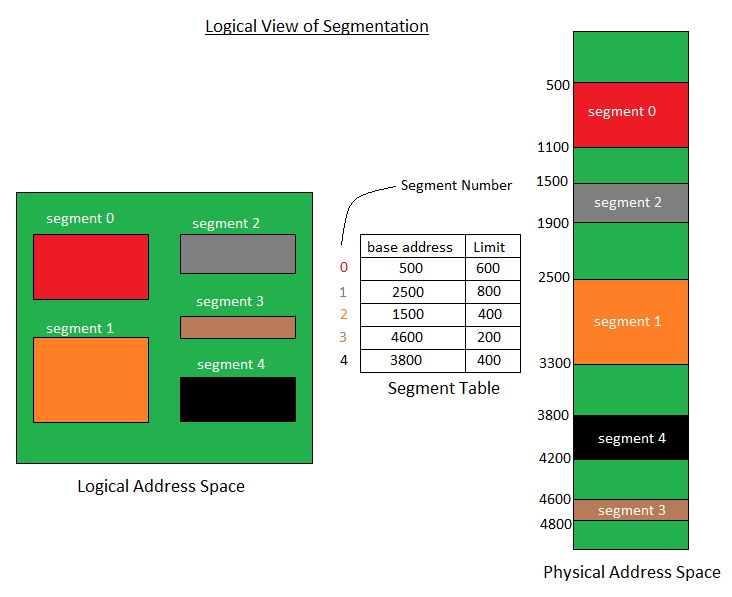
Translation of Two dimensional Logical Address to one dimensional Physical Address.
Segment number (s): Number of bits required to represent the segment.
Segment offset (d): Number of bits required to represent the size of the segment.
Advantages of Segmentation –
No Internal fragmentation.
Segment Table consumes less space in comparison to Page table in paging.
Disadvantage of Segmentation –
As processes are loaded and removed from the memory, the free memory space is broken into little pieces, causing External fragmentation
Virtual Memory in Operating System
Virtual Memory is a storage allocation scheme in which secondary memory can be addressed as though it were part of the main memory. The addresses a program may use to reference memory are distinguished from the addresses the memory system uses to identify physical storage sites, and program-generated addresses are translated automatically to the corresponding machine addresses.
The size of virtual storage is limited by the addressing scheme of the computer system and the amount of secondary memory is available not by the actual number of the main storage locations.
It is a technique that is implemented using both hardware and software. It maps memory addresses used by a program, called virtual addresses, into physical addresses in computer memory.
All memory references within a process are logical addresses that are dynamically translated into physical addresses at run time. This means that a process can be swapped in and out of the main memory such that it occupies different places in the main memory at different times during the course of execution.
A process may be broken into a number of pieces and these pieces need not be continuously located in the main memory during execution. The combination of dynamic run-time address translation and use of page or segment table permits this.
If these characteristics are present then, it is not necessary that all the pages or segments are present in the main memory during execution. This means that the required pages need to be loaded into memory whenever required. Virtual memory is implemented using Demand Paging or Demand Segmentation.
Demand Paging :
The process of loading the page into memory on demand (whenever page fault occurs) is known as demand paging.
The process includes the following steps :

If the CPU tries to refer to a page that is currently not available in the main memory, it generates an interrupt indicating a memory access fault.
The OS puts the interrupted process in a blocking state. For the execution to proceed the OS must bring the required page into the memory.
The OS will search for the required page in the logical address space.
The required page will be brought from logical address space to physical address space. The page replacement algorithms are used for the decision-making of replacing the page in physical address space.
The page table will be updated accordingly.
The signal will be sent to the CPU to continue the program execution and it will place the process back into the ready state.
Hence whenever a page fault occurs these steps are followed by the operating system and the required page is brought into memory.
Advantages :
More processes may be maintained in the main memory: Because we are going to load only some of the pages of any particular process, there is room for more processes. This leads to more efficient utilization of the processor because it is more likely that at least one of the more numerous processes will be in the ready state at any particular time.
A process may be larger than all of the main memory: One of the most fundamental restrictions in programming is lifted. A process larger than the main memory can be executed because of demand paging. The OS itself loads pages of a process in the main memory as required.
It allows greater multiprogramming levels by using less of the available (primary) memory for each process.
Page Fault Service Time :
The time taken to service the page fault is called page fault service time. The page fault service time includes the time taken to perform all the above six steps.
Let Main memory access time is: m
Page fault service time is: s
Page fault rate is : p
Then, Effective memory access time = (p*s) + (1-p)*m
Thrashing :

At any given time, only a few pages of any process are in the main memory and therefore more processes can be maintained in memory. Furthermore, time is saved because unused pages are not swapped in and out of memory. However, the OS must be clever about how it manages this scheme. In the steady-state practically, all of the main memory will be occupied with process pages, so that the processor and OS have direct access to as many processes as possible. Thus when the OS brings one page in, it must throw another out. If it throws out a page just before it is used, then it will just have to get that page again almost immediately. Too much of this leads to a condition called Thrashing. The system spends most of its time swapping pages rather than executing instructions. So a good page replacement algorithm is required.
In the given diagram, the initial degree of multiprogramming up to some extent of point(lambda), the CPU utilization is very high and the system resources are utilized 100%. But if we further increase the degree of multiprogramming the CPU utilization will drastically fall down and the system will spend more time only on the page replacement and the time is taken to complete the execution of the process will increase. This situation in the system is called thrashing.
Causes of Thrashing :
High degree of multiprogramming : If the number of processes keeps on increasing in the memory then the number of frames allocated to each process will be decreased. So, fewer frames will be available for each process. Due to this, a page fault will occur more frequently and more CPU time will be wasted in just swapping in and out of pages and the utilization will keep on decreasing.
For example:
Let free frames = 400
Case 1: Number of process = 100
Then, each process will get 4 frames.
Case 2: Number of processes = 400
Each process will get 1 frame.
Case 2 is a condition of thrashing, as the number of processes is increased, frames per process are decreased. Hence CPU time will be consumed in just swapping pages.
Lacks of Frames: If a process has fewer frames then fewer pages of that process will be able to reside in memory and hence more frequent swapping in and out will be required. This may lead to thrashing. Hence sufficient amount of frames must be allocated to each process in order to prevent thrashing.
Page Replacement Algorithms in Operating Systems
In an operating system that uses paging for memory management, a page replacement algorithm is needed to decide which page needs to be replaced when new page comes in.
Page Fault – A page fault happens when a running program accesses a memory page that is mapped into the virtual address space, but not loaded in physical memory.
Since actual physical memory is much smaller than virtual memory, page faults happen. In case of page fault, Operating System might have to replace one of the existing pages with the newly needed page. Different page replacement algorithms suggest different ways to decide which page to replace. The target for all algorithms is to reduce the number of page faults.
Page Replacement Algorithms :
1. First In First Out (FIFO) –
This is the simplest page replacement algorithm. In this algorithm, the operating system keeps track of all pages in the memory in a queue, the oldest page is in the front of the queue. When a page needs to be replaced page in the front of the queue is selected for removal.
Example-1Consider page reference string 1, 3, 0, 3, 5, 6 with 3 page frames.Find number of page faults.

Initially all slots are empty, so when 1, 3, 0 came they are allocated to the empty slots —> 3 Page Faults.
when 3 comes, it is already in memory so —> 0 Page Faults.
Then 5 comes, it is not available in memory so it replaces the oldest page slot i.e 1. —>1 Page Fault.
6 comes, it is also not available in memory so it replaces the oldest page slot i.e 3 —>1 Page Fault.
Finally when 3 come it is not available so it replaces 0 1 page fault
Belady’s anomaly – Belady’s anomaly proves that it is possible to have more page faults when increasing the number of page frames while using the First in First Out (FIFO) page replacement algorithm. For example, if we consider reference string 3, 2, 1, 0, 3, 2, 4, 3, 2, 1, 0, 4 and 3 slots, we get 9 total page faults, but if we increase slots to 4, we get 10 page faults.
2. Optimal Page replacement –
In this algorithm, pages are replaced which would not be used for the longest duration of time in the future.
Example-2:Consider the page references 7, 0, 1, 2, 0, 3, 0, 4, 2, 3, 0, 3, 2, with 4 page frame. Find number of page fault.

Initially all slots are empty, so when 7 0 1 2 are allocated to the empty slots —> 4 Page faults
0 is already there so —> 0 Page fault.
when 3 came it will take the place of 7 because it is not used for the longest duration of time in the future.—>1 Page fault.
0 is already there so —> 0 Page fault..
4 will takes place of 1 —> 1 Page Fault.
Now for the further page reference string —> 0 Page fault because they are already available in the memory.
Optimal page replacement is perfect, but not possible in practice as the operating system cannot know future requests. The use of Optimal Page replacement is to set up a benchmark so that other replacement algorithms can be analyzed against it.
3. Least Recently Used –
In this algorithm page will be replaced which is least recently used.
Example-3Consider the page reference string 7, 0, 1, 2, 0, 3, 0, 4, 2, 3, 0, 3, 2 with 4 page frames.Find number of page faults.

Initially all slots are empty, so when 7 0 1 2 are allocated to the empty slots —> 4 Page faults
0 is already their so —> 0 Page fault.
when 3 came it will take the place of 7 because it is least recently used —>1 Page fault
0 is already in memory so —> 0 Page fault.
Allocation of frames in Operating System
An important aspect of operating systems, virtual memory is implemented using demand paging. Demand paging necessitates the development of a page-replacement algorithm and a frame allocation algorithm. Frame allocation algorithms are used if you have multiple processes; it helps decide how many frames to allocate to each process.
There are various constraints to the strategies for the allocation of frames:
You cannot allocate more than the total number of available frames.
At least a minimum number of frames should be allocated to each process. This constraint is supported by two reasons. The first reason is, as less number of frames are allocated, there is an increase in the page fault ratio, decreasing the performance of the execution of the process. Secondly, there should be enough frames to hold all the different pages that any single instruction can reference.
Frame allocation algorithms –
The two algorithms commonly used to allocate frames to a process are:
Equal allocation: In a system with x frames and y processes, each process gets equal number of frames, i.e. x/y. For instance, if the system has 48 frames and 9 processes, each process will get 5 frames. The three frames which are not allocated to any process can be used as a free-frame buffer pool.
Disadvantage: In systems with processes of varying sizes, it does not make much sense to give each process equal frames. Allocation of a large number of frames to a small process will eventually lead to the wastage of a large number of allocated unused frames.
Proportional allocation: Frames are allocated to each process according to the process size.
For a process pi of size si, the number of allocated frames is ai = (si/S)*m, where S is the sum of the sizes of all the processes and m is the number of frames in the system. For instance, in a system with 62 frames, if there is a process of 10KB and another process of 127KB, then the first process will be allocated (10/137)*62 = 4 frames and the other process will get (127/137)*62 = 57 frames.
Advantage: All the processes share the available frames according to their needs, rather than equally.
Global vs Local Allocation –
The number of frames allocated to a process can also dynamically change depending on whether you have used global replacement or local replacement for replacing pages in case of a page fault.
Local replacement: When a process needs a page which is not in the memory, it can bring in the new page and allocate it a frame from its own set of allocated frames only.
Advantage: The pages in memory for a particular process and the page fault ratio is affected by the paging behavior of only that process.
Disadvantage: A low priority process may hinder a high priority process by not making its frames available to the high priority process.
Global replacement: When a process needs a page which is not in the memory, it can bring in the new page and allocate it a frame from the set of all frames, even if that frame is currently allocated to some other process; that is, one process can take a frame from another.
Advantage: Does not hinder the performance of processes and hence results in greater system throughput.
Disadvantage: The page fault ratio of a process can not be solely controlled by the process itself. The pages in memory for a process depends on the paging behavior of other processes as well.
UNIT 2
Process Concept
A process is basically a program in execution. The execution of a process must progress in a sequential fashion.
A process is defined as an entity which represents the basic unit of work to be implemented in the system.
To put it in simple terms, we write our computer programs in a text file and when we execute this program, it becomes a process which performs all the tasks mentioned in the program.
When a program is loaded into the memory and it becomes a process, it can be divided into four sections ─ stack, heap, text and data. The following image shows a simplified layout of a process inside main memory −
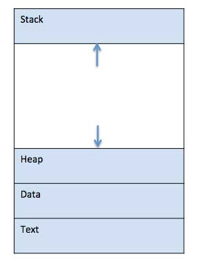
S.N.Component & Description
1
Stack
The process Stack contains the temporary data such as method/function parameters, return address and local variables.
2
Heap
This is dynamically allocated memory to a process during its run time.
3
Text
This includes the current activity represented by the value of Program Counter and the contents of the processor's registers.
4
Data
This section contains the global and static variables.
Process Scheduling
Definition
The process scheduling is the activity of the process manager that handles the removal of the running process from the CPU and the selection of another process on the basis of a particular strategy.
Process scheduling is an essential part of a Multiprogramming operating systems. Such operating systems allow more than one process to be loaded into the executable memory at a time and the loaded process shares the CPU using time multiplexing.
Process Scheduling Queues
The OS maintains all PCBs in Process Scheduling Queues. The OS maintains a separate queue for each of the process states and PCBs of all processes in the same execution state are placed in the same queue. When the state of a process is changed, its PCB is unlinked from its current queue and moved to its new state queue.
The Operating System maintains the following important process scheduling queues −
Job queue − This queue keeps all the processes in the system.
Ready queue − This queue keeps a set of all processes residing in main memory, ready and waiting to execute. A new process is always put in this queue.
Device queues − The processes which are blocked due to unavailability of an I/O device constitute this queue.
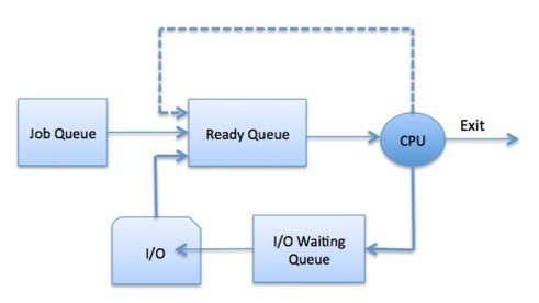
The OS can use different policies to manage each queue (FIFO, Round Robin, Priority, etc.). The OS scheduler determines how to move processes between the ready and run queues which can only have one entry per processor core on the system; in the above diagram, it has been merged with the CPU.
Two-State Process Model
Two-state process model refers to running and non-running states which are described below −
S.N.State & Description
1
Running
When a new process is created, it enters into the system as in the running state.
2
Not Running
Processes that are not running are kept in queue, waiting for their turn to execute. Each entry in the queue is a pointer to a particular process. Queue is implemented by using linked list. Use of dispatcher is as follows. When a process is interrupted, that process is transferred in the waiting queue. If the process has completed or aborted, the process is discarded. In either case, the dispatcher then selects a process from the queue to execute.
Schedulers
Schedulers are special system software which handle process scheduling in various ways. Their main task is to select the jobs to be submitted into the system and to decide which process to run. Schedulers are of three types −
Long-Term Scheduler
Short-Term Scheduler
Medium-Term Scheduler
Long Term Scheduler
It is also called a job scheduler. A long-term scheduler determines which programs are admitted to the system for processing. It selects processes from the queue and loads them into memory for execution. Process loads into the memory for CPU scheduling.
The primary objective of the job scheduler is to provide a balanced mix of jobs, such as I/O bound and processor bound. It also controls the degree of multiprogramming. If the degree of multiprogramming is stable, then the average rate of process creation must be equal to the average departure rate of processes leaving the system.
On some systems, the long-term scheduler may not be available or minimal. Time-sharing operating systems have no long term scheduler. When a process changes the state from new to ready, then there is use of long-term scheduler.
Short Term Scheduler
It is also called as CPU scheduler. Its main objective is to increase system performance in accordance with the chosen set of criteria. It is the change of ready state to running state of the process. CPU scheduler selects a process among the processes that are ready to execute and allocates CPU to one of them.
Short-term schedulers, also known as dispatchers, make the decision of which process to execute next. Short-term schedulers are faster than long-term schedulers.
Medium Term Scheduler
Medium-term scheduling is a part of swapping. It removes the processes from the memory. It reduces the degree of multiprogramming. The medium-term scheduler is in-charge of handling the swapped out-processes.
A running process may become suspended if it makes an I/O request. A suspended processes cannot make any progress towards completion. In this condition, to remove the process from memory and make space for other processes, the suspended process is moved to the secondary storage. This process is called swapping, and the process is said to be swapped out or rolled out. Swapping may be necessary to improve the process mix.
Comparison among Scheduler
S.N.Long-Term SchedulerShort-Term SchedulerMedium-Term Scheduler
1 It is a job scheduler It is a CPU scheduler It is a process swapping scheduler.
2 Speed is lesser than short term scheduler Speed is fastest among other two Speed is in between both short and long term scheduler.
3 It controls the degree of multiprogramming It provides lesser control over degree of multiprogramming It reduces the degree of multiprogramming.
4 It is almost absent or minimal in time sharing system It is also minimal in time sharing system It is a part of Time sharing systems.
5 It selects processes from pool and loads them into memory for execution It selects those processes which are ready to execute It can re-introduce the process into memory and execution can be continued.
Scheduling algorithms
A Process Scheduler schedules different processes to be assigned to the CPU based on particular scheduling algorithms. There are six popular process scheduling algorithms which we are going to discuss in this chapter −
First-Come, First-Served (FCFS) Scheduling
Shortest-Job-Next (SJN) Scheduling
Priority Scheduling
Shortest Remaining Time
Round Robin(RR) Scheduling
Multiple-Level Queues Scheduling
These algorithms are either non-preemptive or preemptive. Non-preemptive algorithms are designed so that once a process enters the running state, it cannot be preempted until it completes its allotted time, whereas the preemptive scheduling is based on priority where a scheduler may preempt a low priority running process anytime when a high priority process enters into a ready state.
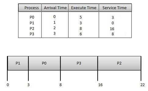
First Come First Serve (FCFS)
Jobs are executed on first come, first serve basis.
It is a non-preemptive, pre-emptive scheduling algorithm.
Easy to understand and implement.
Its implementation is based on FIFO queue.
Poor in performance as average wait time is high.
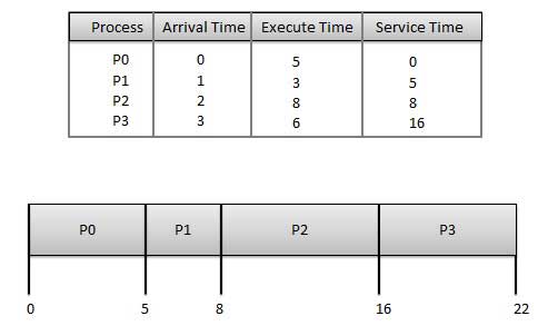
Wait time of each process is as follows −
ProcessWait Time : Service Time - Arrival Time
P0 0 - 0 = 0
P1 5 - 1 = 4
P2 8 - 2 = 6
P3 16 - 3 = 13
Average Wait Time: (0+4+6+13) / 4 = 5.75
Shortest Job Next (SJN)
This is also known as shortest job first, or SJF
This is a non-preemptive, pre-emptive scheduling algorithm.
Best approach to minimize waiting time.
Easy to implement in Batch systems where required CPU time is known in advance.
Impossible to implement in interactive systems where required CPU time is not known.
The processer should know in advance how much time process will take.
Given: Table of processes, and their Arrival time, Execution time
ProcessArrival TimeExecution TimeService Time
P0 0 5 0
P1 1 3 5
P2 2 8 14
P3 3 6 8
Waiting time of each process is as follows −
ProcessWaiting Time
P0 0 - 0 = 0
P1 5 - 1 = 4
P2 14 - 2 = 12
P3 8 - 3 = 5
Average Wait Time: (0 + 4 + 12 + 5)/4 = 21 / 4 = 5.25
Priority Based Scheduling
Priority scheduling is a non-preemptive algorithm and one of the most common scheduling algorithms in batch systems.
Each process is assigned a priority. Process with highest priority is to be executed first and so on.
Processes with same priority are executed on first come first served basis.
Priority can be decided based on memory requirements, time requirements or any other resource requirement.
Given: Table of processes, and their Arrival time, Execution time, and priority. Here we are considering 1 is the lowest priority.
ProcessArrival TimeExecution TimePriorityService Time
P0 0 5 1 0
P1 1 3 2 11
P2 2 8 1 14
P3 3 6 3 5
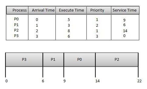
Waiting time of each process is as follows −
ProcessWaiting Time
P0 0 - 0 = 0
P1 11 - 1 = 10
P2 14 - 2 = 12
P3 5 - 3 = 2
Average Wait Time: (0 + 10 + 12 + 2)/4 = 24 / 4 = 6
Shortest Remaining Time
Shortest remaining time (SRT) is the preemptive version of the SJN algorithm.
The processor is allocated to the job closest to completion but it can be preempted by a newer ready job with shorter time to completion.
Impossible to implement in interactive systems where required CPU time is not known.
It is often used in batch environments where short jobs need to give preference.
Round Robin Scheduling
Round Robin is the preemptive process scheduling algorithm.
Each process is provided a fix time to execute, it is called a quantum.
Once a process is executed for a given time period, it is preempted and other process executes for a given time period.
Context switching is used to save states of preempted processes.
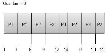
Wait time of each process is as follows −
ProcessWait Time : Service Time - Arrival Time
P0 (0 - 0) + (12 - 3) = 9
P1 (3 - 1) = 2
P2 (6 - 2) + (14 - 9) + (20 - 17) = 12
P3 (9 - 3) + (17 - 12) = 11
Average Wait Time: (9+2+12+11) / 4 = 8.5
Multiple-Level Queues Scheduling
Multiple-level queues are not an independent scheduling algorithm. They make use of other existing algorithms to group and schedule jobs with common characteristics.
Multiple queues are maintained for processes with common characteristics.
Each queue can have its own scheduling algorithms.
Priorities are assigned to each queue.
For example, CPU-bound jobs can be scheduled in one queue and all I/O-bound jobs in another queue. The Process Scheduler then alternately selects jobs from each queue and assigns them to the CPU based on the algorithm assigned to the queue.
Multi-Threading
What is Thread?
A thread is a flow of execution through the process code, with its own program counter that keeps track of which instruction to execute next, system registers which hold its current working variables, and a stack which contains the execution history.
A thread shares with its peer threads few information like code segment, data segment and open files. When one thread alters a code segment memory item, all other threads see that.
A thread is also called a lightweight process. Threads provide a way to improve application performance through parallelism. Threads represent a software approach to improving performance of operating system by reducing the overhead thread is equivalent to a classical process.
Each thread belongs to exactly one process and no thread can exist outside a process. Each thread represents a separate flow of control. Threads have been successfully used in implementing network servers and web server. They also provide a suitable foundation for parallel execution of applications on shared memory multiprocessors. The following figure shows the working of a single-threaded and a multithreaded process.
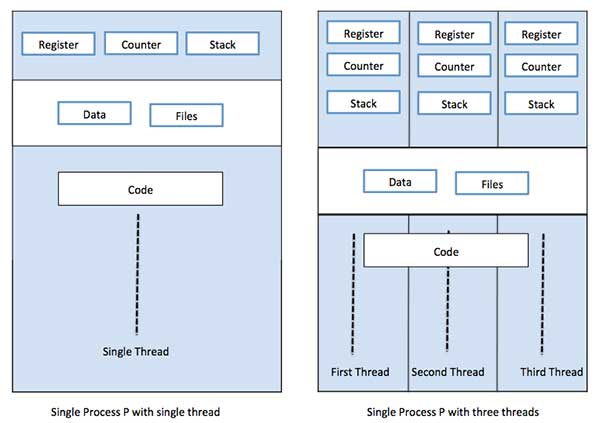
Difference between Process and Thread
S.N.ProcessThread
1 Process is heavy weight or resource intensive. Thread is light weight, taking lesser resources than a process.
2 Process switching needs interaction with operating system. Thread switching does not need to interact with operating system.
3 In multiple processing environments, each process executes the same code but has its own memory and file resources. All threads can share same set of open files, child processes.
4 If one process is blocked, then no other process can execute until the first process is unblocked. While one thread is blocked and waiting, a second thread in the same task can run.
5 Multiple processes without using threads use more resources. Multiple threaded processes use fewer resources.
6 In multiple processes each process operates independently of the others. One thread can read, write or change another thread's data.
Advantages of Thread
Threads minimize the context switching time.
Use of threads provides concurrency within a process.
Efficient communication.
It is more economical to create and context switch threads.
Threads allow utilization of multiprocessor architectures to a greater scale and efficiency.
Types of Thread
Threads are implemented in following two ways −
User Level Threads − User managed threads.
Kernel Level Threads − Operating System managed threads acting on kernel, an operating system core.
User Level Threads
In this case, the thread management kernel is not aware of the existence of threads. The thread library contains code for creating and destroying threads, for passing message and data between threads, for scheduling thread execution and for saving and restoring thread contexts. The application starts with a single thread.
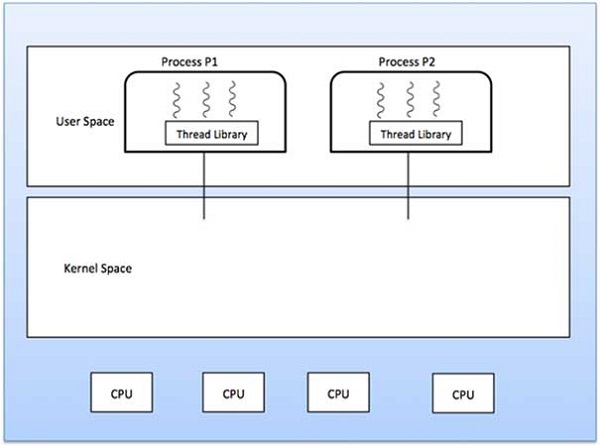
Advantages
Thread switching does not require Kernel mode privileges.
User level thread can run on any operating system.
Scheduling can be application specific in the user level thread.
User level threads are fast to create and manage.
Disadvantages
In a typical operating system, most system calls are blocking.
Multithreaded application cannot take advantage of multiprocessing.
Process Synchronization
On the basis of synchronization, processes are categorized as one of the following two types:
Independent Process : Execution of one process does not affects the execution of other processes.
Cooperative Process : Execution of one process affects the execution of other processes.
Process synchronization problem arises in the case of Cooperative process also because resources are shared in Cooperative processes.
Race Condition
When more than one processes are executing the same code or accessing the same memory or any shared variable in that condition there is a possibility that the output or the value of the shared variable is wrong so for that all the processes doing the race to say that my output is correct this condition known as a race condition. Several processes access and process the manipulations over the same data concurrently, then the outcome depends on the particular order in which the access takes place.
A race condition is a situation that may occur inside a critical section. This happens when the result of multiple thread execution in the critical section differs according to the order in which the threads execute.
Race conditions in critical sections can be avoided if the critical section is treated as an atomic instruction. Also, proper thread synchronization using locks or atomic variables can prevent race conditions.
Critical Section Problem
Critical section is a code segment that can be accessed by only one process at a time. Critical section contains shared variables which need to be synchronized to maintain consistency of data variables.
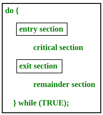
In the entry section, the process requests for entry in the Critical Section.
Any solution to the critical section problem must satisfy three requirements:
Mutual Exclusion : If a process is executing in its critical section, then no other process is allowed to execute in the critical section.
Progress : If no process is executing in the critical section and other processes are waiting outside the critical section, then only those processes that are not executing in their remainder section can participate in deciding which will enter in the critical section next, and the selection can not be postponed indefinitely.
Bounded Waiting : A bound must exist on the number of times that other processes are allowed to enter their critical sections after a process has made a request to enter its critical section and before that request is granted.
Critical Section in Synchronization
Critical Section:
When more than one processes access a same code segment that segment is known as critical section. Critical section contains shared variables or resources which are needed to be synchronized to maintain consistency of data variable.
In simple terms a critical section is group of instructions/statements or region of code that need to be executed atomically (read this post for atomicity), such as accessing a resource (file, input or output port, global data, etc.).
In concurrent programming, if one thread tries to change the value of shared data at the same time as another thread tries to read the value (i.e. data race across threads), the result is unpredictable.
The access to such shared variable (shared memory, shared files, shared port, etc…) to be synchronized. Few programming languages have built-in support for synchronization.
Semaphores in Process Synchronization
Semaphore was proposed by Dijkstra in 1965 which is a very significant technique to manage concurrent processes by using a simple integer value, which is known as a semaphore. Semaphore is simply an integer variable that is shared between threads. This variable is used to solve the critical section problem and to achieve process synchronization in the multiprocessing environment.
Semaphores are of two types:
Binary Semaphore –
This is also known as mutex lock. It can have only two values – 0 and 1. Its value is initialized to 1. It is used to implement the solution of critical section problems with multiple processes.
Counting Semaphore –
Its value can range over an unrestricted domain. It is used to control access to a resource that has multiple instances.
First, look at two operations that can be used to access and change the value of the semaphore variable.
Problem in this implementation of semaphore :
The main problem with semaphores is that they require busy waiting, If a process is in the critical section, then other processes trying to enter critical section will be waiting until the critical section is not occupied by any process.
Whenever any process waits then it continuously checks for semaphore value (look at this line while (s==0); in P operation) and waste CPU cycle.
Dining Philosopher Problem Using Semaphores
The Dining Philosopher Problem – The Dining Philosopher Problem states that K philosophers seated around a circular table with one chopstick between each pair of philosophers. There is one chopstick between each philosopher. A philosopher may eat if he can pick up the two chopsticks adjacent to him. One chopstick may be picked up by any one of its adjacent followers but not both.
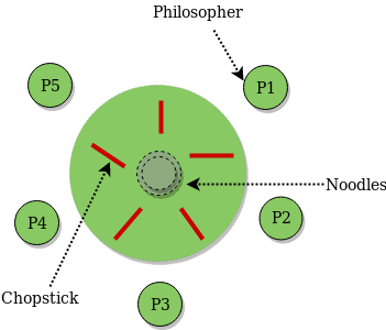
Semaphore Solution to Dining Philosopher –
Each philosopher is represented by the following pseudocode:
process P[i]
while true do
{ THINK;
PICKUP(CHOPSTICK[i], CHOPSTICK[i+1 mod 5]);
EAT;
PUTDOWN(CHOPSTICK[i], CHOPSTICK[i+1 mod 5])
}
There are three states of the philosopher: THINKING, HUNGRY, and EATING. Here there are two semaphores: Mutex and a semaphore array for the philosophers. Mutex is used such that no two philosophers may access the pickup or putdown at the same time. The array is used to control the behavior of each philosopher. But, semaphores can result in deadlock due to programming errors.
Sleeping Barber problem in Process Synchronization
Problem : The analogy is based upon a hypothetical barber shop with one barber. There is a barber shop which has one barber, one barber chair, and n chairs for waiting for customers if there are any to sit on the chair.
If there is no customer, then the barber sleeps in his own chair.
When a customer arrives, he has to wake up the barber.
If there are many customers and the barber is cutting a customer’s hair, then the remaining customers either wait if there are empty chairs in the waiting room or they leave if no chairs are empty.
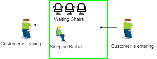
Solution : The solution to this problem includes three semaphores.First is for the customer which counts the number of customers present in the waiting room (customer in the barber chair is not included because he is not waiting). Second, the barber 0 or 1 is used to tell whether the barber is idle or is working, And the third mutex is used to provide the mutual exclusion which is required for the process to execute. In the solution, the customer has the record of the number of customers waiting in the waiting room if the number of customers is equal to the number of chairs in the waiting room then the upcoming customer leaves the barbershop.
Introduction of Deadlock in Operating System
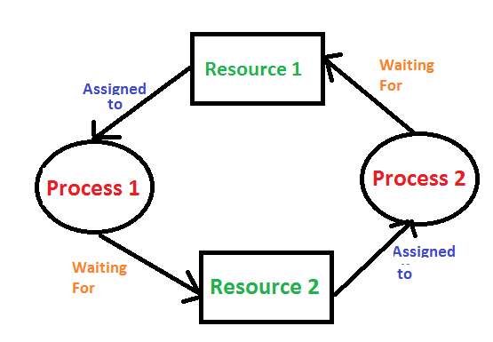
Deadlock is a situation where a set of processes are blocked because each process is holding a resource and waiting for another resource acquired by some other process.
Consider an example when two trains are coming toward each other on the same track and there is only one track, none of the trains can move once they are in front of each other. A similar situation occurs in operating systems when there are two or more processes that hold some resources and wait for resources held by other(s). For example, in the below diagram, Process 1 is holding Resource 1 and waiting for resource 2 which is acquired by process 2, and process 2 is waiting for resource 1.
Deadlock can arise if the following four conditions hold simultaneously (Necessary Conditions)
Mutual Exclusion: One or more than one resource are non-shareable (Only one process can use at a time)
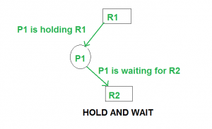
Hold and Wait: A process is holding at least one resource and waiting for resources.
No Preemption: A resource cannot be taken from a process unless the process releases the resource.
Circular Wait: A set of processes are waiting for each other in circular form.
Methods for handling deadlock
There are three ways to handle deadlock
1) Deadlock prevention or avoidance: The idea is to not let the system into a deadlock state.
One can zoom into each category individually, Prevention is done by negating one of above mentioned necessary conditions for deadlock.
Avoidance is kind of futuristic in nature. By using strategy of “Avoidance”, we have to make an assumption. We need to ensure that all information about resources which process will need are known to us prior to execution of the process. We use Banker’s algorithm (Which is in-turn a gift from Dijkstra) in order to avoid deadlock.
2) Deadlock detection and recovery: Let deadlock occur, then do preemption to handle it once occurred.
3) Ignore the problem altogether: If deadlock is very rare, then let it happen and reboot the system. This is the approach that both Windows and UNIX take.
Deadlock Detection Algorithm
If a system does not employ either a deadlock prevention or deadlock avoidance algorithm then a deadlock situation may occur. In this case-
Apply an algorithm to examine state of system to determine whether deadlock has occurred or not.
Apply an algorithm to recover from the deadlock. For more refer- Deadlock Recovery
Deadlock Avoidance Algorithm/ Bankers Algorithm:
The algorithm employs several times varying data structures:
Available –
A vector of length m indicates the number of available resources of each type.
Allocation –
An n*m matrix defines the number of resources of each type currently allocated to a process. Column represents resource and rows represent process.
Request –
An n*m matrix indicates the current request of each process. If request[i][j] equals k then process Pi is requesting k more instances of resource type Rj.
This algorithm has already been discussed here
Now, Bankers algorithm includes a Safety Algorithm / Deadlock Detection Algorithm
The algorithm for finding out whether a system is in a safe state can be described as follows:
Steps of Algorithm:
Let Work and Finish be vectors of length m and n respectively. Initialize Work= Available. For i=0, 1, …., n-1, if Requesti = 0, then Finish[i] = true; otherwise, Finish[i]= false.
Find an index i such that both
a) Finish[i] == false
b) Requesti <= Work
If no such i exists go to step 4.
Work= Work+ Allocationi
Finish[i]= true
Go to Step 2.
If Finish[i]== false for some i, 0<=i<n, then the system is in a deadlocked state. Moreover, if Finish[i]==false the process Pi is deadlocked.
For example,
In this, Work = [0, 0, 0] &
Finish = [false, false, false, false, false]
i=0 is selected as both Finish[0] = false and [0, 0, 0]<=[0, 0, 0].
Work =[0, 0, 0]+[0, 1, 0] =>[0, 1, 0] &
Finish = [true, false, false, false, false].
i=2 is selected as both Finish[2] = false and [0, 0, 0]<=[0, 1, 0].
Work =[0, 1, 0]+[3, 0, 3] =>[3, 1, 3] &
Finish = [true, false, true, false, false].
i=1 is selected as both Finish[1] = false and [2, 0, 2]<=[3, 1, 3].
Work =[3, 1, 3]+[2, 0, 0] =>[5, 1, 3] &
Finish = [true, true, true, false, false].
i=3 is selected as both Finish[3] = false and [1, 0, 0]<=[5, 1, 3].
Work =[5, 1, 3]+[2, 1, 1] =>[7, 2, 4] &
Finish = [true, true, true, true, false].
i=4 is selected as both Finish[4] = false and [0, 0, 2]<=[7, 2, 4].
Work =[7, 2, 4]+[0, 0, 2] =>[7, 2, 6] &
Finish = [true, true, true, true, true].
Since Finish is a vector of all true it means there is no deadlock in this example.
Deadlock Detection And Recovery
Deadlock Detection :
1. If resources have a single instance –
In this case for Deadlock detection, we can run an algorithm to check for the cycle in the Resource Allocation Graph. The presence of a cycle in the graph is a sufficient condition for deadlock.

2. In the above diagram, resource 1 and resource 2 have single instances. There is a cycle R1 → P1 → R2 → P2. So, Deadlock is Confirmed.
3. If there are multiple instances of resources –
Detection of the cycle is necessary but not sufficient condition for deadlock detection, in this case, the system may or may not be in deadlock varies according to different situations.
Deadlock Recovery :
A traditional operating system such as Windows doesn’t deal with deadlock recovery as it is a time and space-consuming process. Real-time operating systems use Deadlock recovery.
Killing the process –
Killing all the processes involved in the deadlock. Killing process one by one. After killing each process check for deadlock again keep repeating the process till the system recovers from deadlock. Killing all the processes one by one helps a system to break circular wait condition.
Resource Preemption –
Resources are preempted from the processes involved in the deadlock, preempted resources are allocated to other processes so that there is a possibility of recovering the system from deadlock. In this case, the system goes into starvation.
Deadlock Prevention And Avoidance
Deadlock Characteristics
As discussed in the previous post, deadlock has following characteristics.
Mutual Exclusion
Hold and Wait
No preemption
Circular wait
Deadlock Prevention
We can prevent Deadlock by eliminating any of the above four conditions.
Eliminate Mutual Exclusion
It is not possible to dis-satisfy the mutual exclusion because some resources, such as the tape drive and printer, are inherently non-shareable.
Eliminate Hold and wait
Allocate all required resources to the process before the start of its execution, this way hold and wait condition is eliminated but it will lead to low device utilization. for example, if a process requires printer at a later time and we have allocated printer before the start of its execution printer will remain blocked till it has completed its execution.
The process will make a new request for resources after releasing the current set of resources. This solution may lead to starvation.
Eliminate No Preemption
Preempt resources from the process when resources required by other high priority processes.
Eliminate Circular Wait
Each resource will be assigned with a numerical number. A process can request the resources increasing/decreasing. order of numbering.
For Example, if P1 process is allocated R5 resources, now next time if P1 ask for R4, R3 lesser than R5 such request will not be granted, only request for resources more than R5 will be granted.
Deadlock Avoidance
Deadlock avoidance can be done with Banker’s Algorithm.
Banker’s Algorithm
Bankers’s Algorithm is resource allocation and deadlock avoidance algorithm which test all the request made by processes for resources, it checks for the safe state, if after granting request system remains in the safe state it allows the request and if there is no safe state it doesn’t allow the request made by the process.
Inputs to Banker’s Algorithm:
Max need of resources by each process.
Currently, allocated resources by each process.
Max free available resources in the system.
The request will only be granted under the below condition:
If the request made by the process is less than equal to max need to that process.
If the request made by the process is less than equal to the freely available resource in the system.
Example: Total resources in system:
A B C D
6 5 7 6
Available system resources are:
A B C D
3 1 1 2
Processes (currently allocated resources):
A B C D
P1 1 2 2 1
P2 1 0 3 3
P3 1 2 1 0
Processes (maximum resources):
A B C D
P1 3 3 2 2
P2 1 2 3 4
P3 1 3 5 0
Need = maximum resources - currently allocated resources.
Processes (need resources):
A B C D
P1 2 1 0 1
P2 0 2 0 1
P3 0 1 4 0
Note: Deadlock prevention is more strict than Deadlock Avoidance.
UNIT 3
Device Management
Device management in an operating system means controlling the Input/Output
devices like disk, microphone, keyboard, printer, magnetic tape, USB ports,
camcorder, scanner, other accessories, and supporting units like supporting
units control channels. A process may require various resources, including
main memory, file access, and access to disk drives, and others. If resources
are available, they could be allocated, and control returned to the CPU.
Otherwise, the procedure would have to be postponed until adequate
resources become available. The system has multiple devices, and in order to
handle these physical or virtual devices, the operating system requires a separate
program known as an ad device controller. It also determines whether the
requested device is available.
The fundamentals of I/O devices may be divided into three categories:
Boot Device
Character Device
Network Device
Boot Device
It stores data in fixed-size blocks, each with its unique address.
For example- Disks.
Character Device
It transmits or accepts a stream of characters, none of which can be addressed
individually. For instance, keyboards, printers, etc.
Network Device
It is used for transmitting the data packets.
Functions of the device management in the operating system
The operating system (OS) handles communication with the devices via their drivers. The OS component gives a uniform interface for accessing devices with various physical features. There are various functions of device management in the operating system. Some of them are as follows:
It keeps track of data, status, location, uses, etc. The file system is a term used to define a group of facilities.
It enforces the pre-determined policies and decides which process receives the device when and for how long.
It improves the performance of specific devices.
It monitors the status of every device, including printers, storage drivers, and other devices.
It allocates and effectively deallocates the device. De-allocating differentiates the devices at two levels: first, when an I/O command is issued and temporarily freed. Second, when the job is completed, and the device is permanently release
Types of devices
There are three types of Operating system peripheral devices: dedicated, shared, and virtual. These are as follows:
1. Dedicated Device
In device management, some devices are allocated or assigned to only one
task at a time until that job releases them. Devices such as plotters, printers,
tape drivers, and other similar devices necessitate such an allocation
mechanism because it will be inconvenient if multiple people share them
simultaneously. The disadvantage of such devices is the inefficiency caused
by allocating the device to a single user for the whole duration of task execution,
even if the device is not used 100% of the time.
2. Shared Devices
These devices could be assigned to a variety of processes.
By interleaving their requests, disk-DASD could be shared by multiple
processes simultaneously. The Device Manager carefully controls the
interleaving, and pre-determined policies must resolve all difficulties.
3. Virtual Devices
Virtual devices are a hybrid of the two devices, and they are dedicated devices
that have been transformed into shared devices. For example, a printer can be
transformed into a shareable device by using a spooling program that redirects all print requests to a disk. A print job is not sent directly to the printer; however, it is routed to the disk until it is fully prepared with all of the required sequences and formatting, at which point it is transmitted to the printers. The approach can transform a single printer into
numerous virtual printers, improving performance and ease of use.
Features of Device Management
Here, you will learn the features of device management in the operating system. Various features of the device management are as follows:
The OS interacts with the device controllers via the device drivers while allocating the device to the multiple processes executing on the system.
Device drivers can also be thought of as system software programs that bridge processes and device controllers.
The device management function's other key job is to implement the API.
Device drivers are software programs that allow an operating system to control the operation of numerous devices effectively.
The device controller used in device management operations mainly contains three registers: command, status, and data.
Buffering in Operating System
The buffer is an area in the main memory used to store or hold the data temporarily.
In other words, buffer temporarily stores data transmitted from one place to another
, either between two devices or an application. The act of storing data temporarily in
the buffer is called buffering.A buffer may be used when moving data between
processes within a computer.
Buffers can be implemented in a fixed memory location in hardware or by using a
virtual data buffer in software, pointing at a location in the physical memory.
In all cases, the data in a data buffer are stored on a physical storage medium.
Most buffers are implemented in software, which typically uses the faster RAM
to store temporary data due to the much faster access time than hard disk drives.
Buffers are typically used when there is a difference between the rate of received
data and the rate of processed data, for example, in a printer spooler or online video
streaming.
A buffer often adjusts timing by implementing a queue or FIFO algorithm in memory,
simultaneously writing data into the queue at one rate and reading it at another rate.
Types of Buffering
There are three main types of buffering in the operating system, such as:
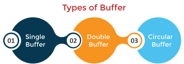
1. Single Buffer
In Single Buffering, only one buffer is used to transfer the data between two devices.
The producer produces one block of data into the buffer. After that, the consumer
consumes the buffer. Only when the buffer is empty, the processor again produces the
data.
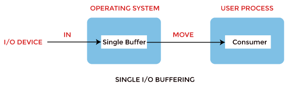
Block oriented device: The following operations are performed in the block-oriented device,
System buffer takes the input.
After taking the input, the block gets transferred to the user space and then requests another block.
Two blocks work simultaneously. When the user processes one block of data, the next block is being read in.
OS can swap the processes.
OS can record the data of the system buffer to user processes.
Stream oriented device: It performed the following operations, such as:
Line-at a time operation is used for scroll made terminals. The user inputs one line at a time, with a carriage return waving at the end of a line.
Byte-at a time operation is used on forms mode, terminals when each keystroke is significant.
2. Double Buffer
In Double Buffering, two schemes or two buffers are used in the place of one. In this buffering, the producer produces one buffer while the consumer consumes another buffer simultaneously. So, the producer not needs to wait for filling the buffer. Double buffering is also known as buffer swapping.
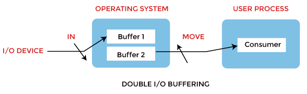
Block oriented: This is how a double buffer works. There are two buffers in the system.
The driver or controller uses one buffer to store data while waiting for it to be taken by a higher hierarchy level.
Another buffer is used to store data from the lower-level module.
A major disadvantage of double buffering is that the complexity of the process gets increased.
If the process performs rapid bursts of I/O, then using double buffering may be deficient.
Stream oriented: It performs these operations, such as:
Line- at a time I/O, the user process does not need to be suspended for input or output unless the process runs ahead of the double buffer.
Byte- at time operations, double buffer offers no advantage over a single buffer of twice the length.
3. Circular Buffer
When more than two buffers are used, the buffers' collection is called a circular buffer. Each buffer is being one unit in the circular buffer. The data transfer rate will increase using the circular buffer rather than the double buffering.
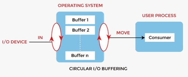
In this, the data do not directly pass from the producer to the consumer because the data would change due to overwriting of buffers before consumed.
The producer can only fill up to buffer x-1 while data in buffer x is waiting to be consumed.
How Buffering Works
In an operating system, buffer works in the following way:
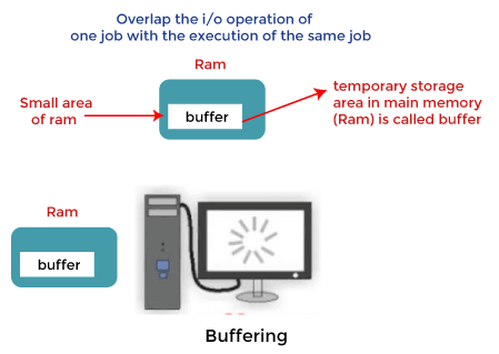
Buffering is done to deal effectively with a speed mismatch between the producer and consumer of the data stream.
A buffer is produced in the main memory to heap up the bytes received from the modem.
After receiving the data in the buffer, the data get transferred to a disk from the buffer in a single operation.
This process of data transfer is not instantaneous. Therefore the modem needs another buffer to store additional incoming data.
When the first buffer got filled, then it is requested to transfer the data to disk.
The modem then fills the additional incoming data in the second buffer while the data in the first buffer gets transferred to the disk.
When both the buffers completed their tasks, the modem switches back to the first buffer while the data from the second buffer gets transferred to the disk.
Two buffers disintegrate the producer and the data consumer, thus minimising the time requirements between them.
Buffering also provides variations for devices that have different data transfer sizes.
Advantages of Buffer
Buffering plays a very important role in any operating system during the execution of any process or task. It has the following advantages.
The use of buffers allows uniform disk access. It simplifies system design.
The system places no data alignment restrictions on user processes doing I/O.
By copying data from user buffers to system buffers and vice versa, the kernel eliminates the need for special alignment of user buffers, making user programs simpler and more portable.
The use of the buffer can reduce the amount of disk traffic, thereby increasing overall system throughput and decreasing response time.
The buffer algorithms help ensure file system integrity.
Disadvantages of Buffer
Buffers are not better in all respects. Therefore, there are a few disadvantages as follows, such as:
It is costly and impractical to have the buffer be the exact size required to hold the number of elements. Thus, the buffer is slightly larger most of the time, with the rest of the space being wasted.
Buffers have a fixed size at any point in time. When the buffer is full, it must be reallocated with a larger size, and its elements must be moved. Similarly, when the number of valid elements in the buffer is significantly smaller than its size, the buffer must be reallocated with a smaller size and elements be moved to avoid too much waste.
Use of the buffer requires an extra data copy when reading and writing to and from user processes. When transmitting large amounts of data, the extra copy slows down performance.
Swapping in Operating System
Swapping is a memory management scheme in which any process can be temporarily swapped from main memory to secondary memory so that the main memory can be made available for other processes. It is used to improve main memory utilization. In secondary memory, the place where the swapped-out process is stored is called swap space.
The purpose of the swapping in operating system
is to access the data present in the hard disk and bring it to RAM
so that the application programs can use it. The thing to remember is that swapping is used only when data is not present in RAM
.
Although the process of swapping affects the performance of the system, it helps to run larger and more than one process. This is the reason why swapping is also referred to as memory compaction.
The concept of swapping has divided into two more concepts: Swap-in and Swap-out.
Swap-out is a method of removing a process from RAM and adding it to the hard disk.
Swap-in is a method of removing a program from a hard disk and putting it back into the main memory or RAM.
Advantages of Swapping
It helps the CPU to manage multiple processes within a single main memory.
It helps to create and use virtual memory.
Swapping allows the CPU to perform multiple tasks simultaneously. Therefore, processes do not have to wait very long before they are executed.
It improves the main memory utilization.
Disadvantages of Swapping
If the computer system loses power, the user may lose all information related to the program in case of substantial swapping activity.
If the swapping algorithm is not good, the composite method can increase the number of Page Fault and decrease the overall processing performance.
Swap-Space Management :
Swap-Swap management is another low-level task of the operating system. Disk space is used as an extension of main memory by the virtual memory. As we know the fact that disk access is much slower than memory access, In the swap-space management we are using disk space, so it will significantly decreases system performance. Basically, in all our systems we require the best throughput, so the goal of this swap-space implementation is to provide the virtual memory the best throughput. In these article, we are going to discuss how swap space is used, where swap space is located on disk, and how swap space is managed.
Swap-Space Use :
Swap-space is used by the different operating-system in various ways. The systems which are implementing swapping may use swap space to hold the entire process which may include image, code and data segments. Paging systems may simply store pages that have been pushed out of the main memory. The need of swap space on a system can vary from a megabytes to gigabytes but it also depends on the amount of physical memory, the virtual memory it is backing and the way in which it is using the virtual memory.
It is safer to overestimate than to underestimate the amount of swap space required, because if a system runs out of swap space it may be forced to abort the processes or may crash entirely. Overestimation wastes disk space that could otherwise be used for files, but it does not harm other.
Following table shows different system using amount of swap space:
Following table shows different system using amount of swap space:
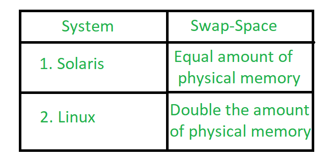
Figure – Different systems using amount of swap-space
Explanation of above table :
Solaris, setting swap space equal to the amount by which virtual memory exceeds page-able physical memory. In the past Linux has suggested setting swap space to double the amount of physical memory. Today, this limitation is gone, and most Linux systems use considerably less swap space.
Including Linux, some operating systems; allow the use of multiple swap spaces, including both files and dedicated swap partitions. The swap spaces are placed on the disk so the load which is on the I/O by the paging and swapping will spread over the system’s bandwidth.
Swap-Space Management: An Example –
The traditional UNIX kernel started with an implementation of swapping that copied entire process between contiguous disk regions and memory. UNIX later evolve to a combination of swapping and paging as paging hardware became available. In Solaris, the designers changed standard UNIX methods to improve efficiency. More changes were made in later versions of Solaris, to improve the efficiency.
Linux is almost similar to Solaris system. In both the systems the swap space is used only for anonymous memory, it is that kind of memory which is not backed by any file. In the Linux system, one or more swap areas are allowed to be established. A swap area may be in either in a swap file on a regular file system or a dedicated file partition.
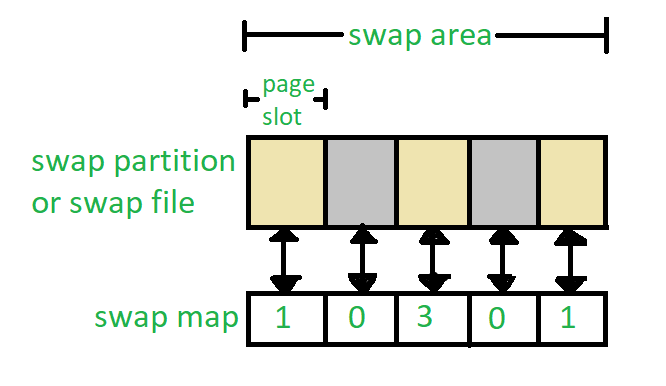
Figure – Data structure for swapping on Linux system
Each swap area consists of 4-KB page slots, which are used to hold the swapped pages.
Associated with each swap area is a swap-map- an array of integers counters,
each corresponding to a page slot in the swap area. If the value of the counter
is 0 it means page slot is occupied by swapped page. The value of counter indicates
the number of mappings to the swapped page. For example, a value 3 indicates that the
swapped page is mapped to the 3 different processes.
File Systems in Operating System
A file is a collection of related information that is recorded on secondary storage.
Or file is a collection of logically related entities. From user’s perspective a file is
the smallest allotment of logical secondary storage
SFS (Symbolic File System)
A command line utility that provides a lightweight setup for organizing and backing up files
SFS stores files from a variety of sources, aka collections, that may include directories and removable media, as symbolic links to the source files. It also stores the metadata of the source files so that files can later be queried without having to plug in the source media.
An SFS is a managed directory which is initialized with the command: sfs init. All commands to be executed in the context of an individual SFS must be run from within the SFS directory tree. Files are added using the command sfs add-col my_collection /path/to/source (add collection). SFS Files are symlinks to source files in added collections. Foreign links and other files can also exist in an SFS but they are not managed by it and are mostly ignored.
Use Cases
Organizing Data Across Discs
SFS was built with the motivation of being able to have a combined view of data stored across multiple discs, organize the data in the view and reflect changes back to source discs. This is an effortless way of organizing content across discs which is otherwise painfully slow and limited as we can operate on a limited number of discs simultaneously and inter disc transfers are very slow. Since all operations in an SFS are performed within the same disc and on symlinks instead of heavy files, they are much faster
Note: To view the content of a file we obviously do need the source to be available. So, if there is a need of viewing file content while organizing them, the source needs to be plugged in which might or might not be appropriate for all use cases. However, SFS makes it easy to query the source of an SFS File when it is needed to be accessed
Backing up Files
While there are lots of ways to make direct backups of directories, an SFS allows you to organize the content while backing them up and potentially saving them to multiple destinations with a single command. For exaback themmple, you might have an SFS in which you add local files, like multimedia and documents, organize them in hierarchies resembling your storage hierarchies, then map the top-level SFS directories to backup destinations and preform the backup with a single save command. Periodically, you will have to synchronize the SFS, sort the newly added local files and rerun the backup.
Decouple Data Storage and View
Data often needs to be stored in a certain way which might not be similar to the hierarchy in which you want to view it. SFS allows you to create a virtual hierarchy for viewing content. For example, consider that you have data saved in a number of discs or directories, organized as music, documents, projects, etc. Your options are either to keep a copy of the important files locally, which we commonly do, or to plugin all the media one by one and search for the files you need, which hopefully no one does. You can instead create an SFS instance, dump all your discs into it, create a directory in the SFS for local files and copy all needed files to your local system. You can search for files in all your discs locally and, periodically, you can update what files to be kept in you local system
.
Basic File System Operations
By considering the fundamental operations we can carry out using file systems, we can see the inherent issues associated with their implementation.
Initialization
We must be able to turn a newly allocated region of a disk into a file system or part of a file system. In any file system there must be at least one fixed location structure. In more traditional unix file systems there are many fixed location structures. These must be laid out in order to allow one to manipulate files. We must also create an empty root (top-level) directory within the file system.
ACCESS CONTROL VERIFICATION
Security policy & verification
A security policy defines security requirements for a given system [Goguen and Meseguer, 1982] Multi-level security (MLS), discretionary access, mandatory access, information-flow, … Verification is a technique that proves whether a policy holds on a system or not
Formal verification
Deductive methods produces formal mathematical correctness using
theorem provers or proof assistances 2) Model checking Exhaustively explores
of all possible behaviors over the state transition system that models program
execution.
Access control:
dynamic vs. static We can divide access control policies into two categories:
1. Dynamic policies: Permissions of the agents depend on the system state and can be changed by the actions of other agents. (PoliVer and DynPAL)
2. Static policies: Access decisions doesn’t change the state of the system.
(Access Control Matrix)
Physical and Logical File Systems
Physical FileLogical FileIt occupies the portion of memory. It contains the original data. It does not occupy memory space. It does not contain data.
A physical file contains one record format. It can contain upto 32 record formats.
It can exist without logical file. It cannot exist without physical file.
If there is a logical file for physical file, the physical file cannot be deleted until and unless we delete the logical file. If there is a logical file for a physical file, the logical file can be deleted without deleting the physical file.
CRTPF command is used to make such object. CRTLF command is used to make such object.
User Interface (UI)
User Interface (UI) defines the way humans interact with the information systems. In Layman’s term, User Interface (UI) is a series of pages, screens, buttons, forms and other visual elements that are used to interact with the device. Every app and every website has a user interface.
User Interface (UI) Design is the creation of graphics, illustrations, and use of photographic artwork and typography to enhance the display and layout of a digital product within its various device views. Interface elements consist of input controls (buttons, drop-down menus, data fields), navigational components (search fields, slider, icons, tags), informational components (progress bars, notifications, message boxes).
File Concept
Computer store information in storage media such as disk, tape drives, and optical disks.
The operating system provides a logical view of the information stored in the disk.
This logical storage unit is a file.
The information stored in files are non-volatile, means they are not lost during power
failures. A file is named collection of related information that is stored on physical storage.
Data cannot be written to a computer unless it is written to a file. A file, in general,.
is a sequence of bits, bytes, lines, or records defined by its owner or creator. The file has a structure defined by its owner or creator and depends on the file type.
Text file – It has a sequence of characters.
Image file – It has visual information such as photographs, vectors art and so on.
Source file – It has subroutines and function that are compiled later.
Object file – It has a sequence of bytes, organized into bytes and used by the linker.
Executable file – The binary code that the loader brings to memory for execution is stored in an exe file
File Access Methods
The information stored in a file must be accessed and read into memory.
Though there are many ways to access a file, some system provides only one method,
other systems provide many methods, out of which you must choose the right one for
the application.
Sequential Access Method
In this method, the information in the file is processed in order, one record after another. For example, compiler and various editors access files in this manner.
The read-next – reads the next portion of a file and updates the file pointer which tracks the I/O location. Similarly, the write-next will write at the end of a file
and advances the pointer to the new end of the file.
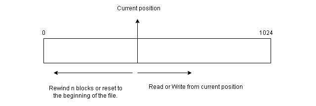 Sequential access to File
The sequential access always reset to the beginning of the file and then starts skipping forward or backward n
records. It works for both sequential devices and random-access devices.
Direct Access Method
The other method for file access is direct access or relative access. For direct access,
the file is viewed as a numbered sequence of blocks or records. This method is based
on the disk model of file. Since disks allow random access to file block.
Structures of Directory in Operating System
A directory is a container that is used to contain folders
and files. It organizes files and folders in a hierarchical
manner.

There are several logical structures of a directory, these are given below.
Single-level directory –
The single-level directory is the simplest directory structure. In it, all files are contained in the same directory which makes it easy to support and understand.
A single level directory has a significant limitation, however, when the number of files increases or when the system has more than one user. Since all the files are in the same directory, they must have a unique name. if two users call their dataset test, then the unique name rule violated.

Advantages:
Since it is a single directory, so its implementation is very easy.
If the files are smaller in size, searching will become faster.
The operations like file creation, searching, deletion, updating are very easy in such a directory structure.
Disadvantages:
There may chance of name collision because two files can have the same name.
Searching will become time taking if the directory is large.
This can not group the same type of files together.
Two-level directory –
As we have seen, a single level directory often leads to confusion
of files names among different users. the solution to this problem
is to create a separate directory for each user.
In the two-level directory structure, each user has their own user
files directory (UFD). The UFDs have similar structures,
but each lists only the files of a single user. system’s master file directory (MFD) is searches whenever a new user id=s logged in. The MFD is indexed by username or account number, and each entry points to the UFD for that user.

Advantages:
We can give full path like /User-name/directory-name/.
Different users can have the same directory as well as the file name.
Searching of files becomes easier due to pathname and user-grouping.
Disadvantages:
A user is not allowed to share files with other users.
Still, it not very scalable, two files of the same type cannot be grouped together in the same user.
Tree-structured directory –
Once we have seen a two-level directory as a tree of height 2, the natural generalization is to extend the directory structure to a tree of arbitrary height.
This generalization allows the user to create their own subdirectories and to organize their files accordingly.

A tree structure is the most common directory structure. The tree has a root directory, and every file in the system has a unique path.
Advantages:
Very general, since full pathname can be given.
Very scalable, the probability of name collision is less.
Searching becomes very easy, we can use both absolute paths as well as relative.
Disadvantages:
Every file does not fit into the hierarchical model, files may be saved into multiple directories.
We can not share files.
It is inefficient, because accessing a file may go under multiple directories.
Acyclic graph directory –
An acyclic graph is a graph with no cycle and allows us to share subdirectories and files. The same file or subdirectories may be in two different directories. It is a natural generalization of the tree-structured directory.
It is used in the situation like when two programmers are working on a joint project and they need to access files. The associated files are stored in a subdirectory, separating them from other projects and files of other programmers since they are working on a joint project so they want the subdirectories to be into their own directories. The common subdirectories should be shared. So here we use Acyclic directories.
It is the point to note that the shared file is not the same as the copy file. If any programmer makes some changes in the subdirectory it will reflect in both subdirectories.

Advantages:
We can share files.
Searching is easy due to different-different paths.
Disadvantages:
We share the files via linking, in case deleting it may create the problem,
If the link is a soft link then after deleting the file we left with a dangling pointer.
In the case of a hard link, to delete a file we have to delete all the references associated with it.
General graph directory structure –
In general graph directory structure, cycles are allowed within a directory structure where multiple directories can be derived from more than one parent directory.
The main problem with this kind of directory structure is to calculate the total size or space that has been taken by the files and directories.

Advantages:
It allows cycles.
It is more flexible than other directories structure.
Disadvantages:
It is more costly than others.
It needs garbage collection.
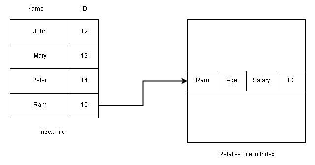 Direct Access Method Using Index
You can read block 34, then read 45, and write in block 78, there is no restriction on the order of access to the file.
The direct access method is used in database management. A query is satisfied immediately by accessing large
amount of information stored in database files directly.
The database maintains an index of blocks which contains the block number. This block can be accessed directly and
information is retrieved.
Consistency Semantics for file sharing
Consistency Semantics is concept which is used by users to check file
systems which are supporting file sharing in their systems. Basically, it is specification to check that how in a single system multiple users are getting access to same file and at same time. They are used to check various things in files, like when will modification by some
user in some file is noticeable to others.
Consistency Semantics is concept which is in a direct relation with
concept named process synchronization algorithms. But
process synchronization algorithms are not used in case of file I/O because of
several issues like great latency, slower rate of transfer of disk
and network.
To access same file by user process is always enclosed between open() and close()
operations. When there are series of access take place for same file, then it makes up
a file session.

1. UNIX Semantics :
The file systems in UNIX uses following consistency semantics –
The file which user is going to be write will be visible to all users who are sharing
that file at that time.
Their is one mode in UNIX semantics to share file is via sharing pointer of current
location. But it will affect all other sharing users.
In this, a file which is shared is associated with a single physical image that is accessed
as an exclusive resources. This single image causes delays in user processes.
2. Session Semantics :
The file system in Andrew uses following consistency semantics.
The file which user is going to be write will not visible to all users who are sharing
that file at that time.
After closing file, changes done to that file by user are only visible only in sessions
starting later. If changes file is already open by other user, then changes will
not be visible to that user.
In this, a file which is shared is associated with a several images and there is no delay
in this because it allows multiple users to perform both read and write accesses
concurrently on their images.
3. Immutable-Shared-Files Semantics :
There seems a unique approach immutable shared files. In this, user are not allowed to modify file, which is declared as shared by its creator.
An Immutable file has two properties which are as follows –
Its name may not be reused.
Its content may not be altered.
In this file system, content of file are fixed. The implementation of semantics in a distributed system is simple, because sharing is disciplined
File Allocation Methods
The allocation methods define how the files are stored in the disk blocks.
There are three main disk space or file allocation methods.
Contiguous Allocation
Linked Allocation
Indexed Allocation
The main idea behind these methods is to provide:
Efficient disk space utilization.
Fast access to the file blocks.
All the three methods have their own advantages and disadvantages as discussed
below:
1. Contiguous Allocation
In this scheme, each file occupies a contiguous set of blocks on the disk. For example,
if a file requires n blocks and is given a block b as the starting location, then the blocks
assigned to the file will be: b, b+1, b+2,……b+n-1. This means that given the starting
block address and the length of the file (in terms of blocks required), we can determine
the blocks occupied by the file.
The directory entry for a file with contiguous allocation contains
Address of starting block
Length of the allocated portion.
The file ‘mail’ in the following figure starts from the block 19 with length = 6 blocks.
Therefore, it occupies 19, 20, 21, 22, 23, 24 blocks.
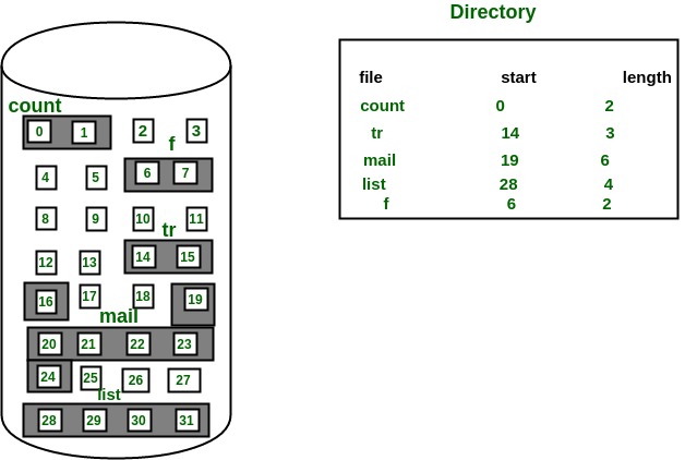
Advantages:
Both the Sequential and Direct Accesses are supported by this. For direct access,
the address of the kth block of the file which starts at block b can easily be obtained
as (b+k).
This is extremely fast since the number of seeks are minimal because of
contiguous allocation of file blocks.
Disadvantages:
This method suffers from both internal and external fragmentation. This makes it
inefficient in terms of memory utilization.
Increasing file size is difficult because it depends on the availability of contiguous
memory at a particular instance.
2. Linked List Allocation
In this scheme, each file is a linked list of disk blocks which need not be contiguous.
The disk blocks can be scattered anywhere on the disk.
The directory entry contains a pointer to the starting and the ending file block.
Each block contains a pointer to the next block occupied by the file.
The file ‘jeep’ in following image shows how the blocks are randomly distributed.
The last block (25) contains -1 indicating a null pointer and does not point to any other
block.
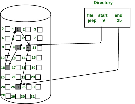
Advantages:
This is very flexible in terms of file size. File size can be increased easily since
the system does not have to look for a contiguous chunk of memory.
This method does not suffer from external fragmentation. This makes it relatively
better in terms of memory utilization.
Disadvantages:
Because the file blocks are distributed randomly on the disk, a large number
of seeks are needed to access every block individually.
This makes linked allocation slower.
It does not support random or direct access. We can not directly access
the blocks of a file. A block k of a file can be accessed by traversing k blocks
sequentially (sequential access ) from the starting block of the file via block pointers.
Pointers required in the linked allocation incur some extra overhead.
3. Indexed Allocation
In this scheme, a special block known as the Index block contains the pointers to all the blocks occupied by a file. Each file has its own index block. The ith entry in the index block contains the disk address of the ith file block. The directory entry contains the address of the index block as shown in the image:
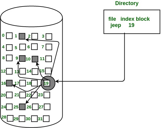
Advantages:
This supports direct access to the blocks occupied by the file and therefore provides fast access to the file blocks.
It overcomes the problem of external fragmentation.
Disadvantages:
The pointer overhead for indexed allocation is greater than linked allocation.
For very small files, say files that expand only 2-3 blocks, the indexed allocation would keep one entire block (index block) for the pointers which is inefficient in terms of memory utilization. However, in linked allocation we lose the space of only 1 pointer per block.
For files that are very large, single index block may not be able to hold all the pointers.
Following mechanisms can be used to resolve this:
Linked scheme: This scheme links two or more index blocks together for holding the pointers. Every index block would then contain a pointer or the address to the next index block.
Multilevel index: In this policy, a first level index block is used to point to the second level index blocks which inturn points to the disk blocks occupied by the file. This can be extended to 3 or more levels depending on the maximum file size.
Combined Scheme: In this scheme, a special block called the Inode (information Node) contains all the information about the file such as the name, size, authority, etc and the remaining space of Inode is used to store the Disk Block addresses which contain the actual file as shown in the image below. The first few of these pointers in Inode point to the direct blocks i.e the pointers contain the addresses of the disk blocks that contain data of the file. The next few pointers point to indirect blocks. Indirect blocks may be single indirect, double indirect or triple indirect. Single Indirect block is the disk block that does not contain the file data but the disk address of the blocks that contain the file data. Similarly, double indirect blocks do not contain the file data but the disk address of the blocks that contain the address of the blocks containing the file data.
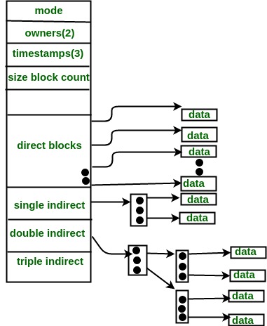
This article is contributed by Saloni Baweja. If you like GeeksforGeeks and would like to contribute, you can also write an article using contribute.geeksforgeeks.org or mail your article to contribute@geeksforgeeks.org. See your article appearing on the GeeksforGeeks main page and help other Geeks.
Please write comments if you find anything incorrect, or you want to share
more information about the topic discussed above.
Free space management in Operating System
The system keeps tracks of the free disk blocks for allocating space to files when they are created. Also, to reuse the space released from deleting the files, free space management becomes crucial. The system maintains a free space list which keeps track of the disk blocks that are not allocated to some file or directory. The free space list can be implemented mainly as:
Bitmap or Bit vector –
A Bitmap or Bit Vector is series or collection of bits where each bit corresponds to a disk block. The bit can take two values: 0 and 1: 0 indicates that the block is allocated and 1 indicates a free block.
The given instance of disk blocks on the disk in Figure 1 (where green blocks are allocated) can be represented by a bitmap of 16 bits as: 0000111000000110.
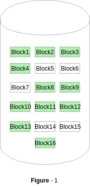
Advantages –
Simple to understand.
Finding the first free block is efficient. It requires scanning the words (a group of 8 bits) in a bitmap for a non-zero word. (A 0-valued word has all bits 0). The first free block is then found by scanning for the first 1 bit in the non-zero word.
The block number can be calculated as:
(number of bits per word) *(number of 0-values words) + offset of bit first bit 1 in the non-zero word .
For the Figure-1, we scan the bitmap sequentially for the first non-zero word.
The first group of 8 bits (00001110) constitute a non-zero word since all bits are not 0. After the non-0 word is found, we look for the first 1 bit. This is the 5th bit of the non-zero word. So, offset = 5.
Therefore, the first free block number = 8*0+5 = 5.
Linked List –
In this approach, the free disk blocks are linked together i.e. a free block contains a pointer to the next free block. The block number of the very first disk block is stored at a separate location on disk and is also cached in memory.
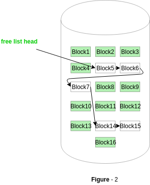
In Figure-2, the free space list head points to Block 5 which points to Block 6, the next free block and so on. The last free block would contain a null pointer indicating the end of free list.
A drawback of this method is the I/O required for free space list traversal.
Grouping –
This approach stores the address of the free blocks in the first free block. The first free block stores the address of some, say n free blocks. Out of these n blocks, the first n-1 blocks are actually free and the last block contains the address of next free n blocks.
An advantage of this approach is that the addresses of a group of free disk blocks can be found easily.
Counting –
This approach stores the address of the first free disk block and a number n of free contiguous disk blocks that follow the first block.
Every entry in the list would contain:
Address of first free disk block
A number n
UNIT 4
Log into and out of your Unix account
Log into Unix
Before beginning, make sure your Caps Lock key is off. On most keyboards it is above your left Shift key. To log into your Unix account:
At the Login: prompt, enter your username.
At the Password: prompt, enter your password. For security reasons, your password does not appear on the screen when you type it. If you enter an incorrect password, you'll be asked to enter your username and password again. (Be aware that the Backspace or Del keys might not work properly while you are entering your password.)
On many systems, a page of information and announcements, called a banner or "message of the day" (MOD), will be displayed on your screen. It notifies you of system changes, scheduled maintenance, and other news.
The following line may appear after the banner: TERM = (vt100)
Normally, you can press Enter to set the correct terminal type. If you know that the suggested terminal type is incorrect, enter the terminal type that your communications program is using. If you are unsure of the correct type, enter vt100.
After a pause, the Unix shell prompt will appear.
You can now enter commands at the Unix prompt.
Log out of Unix
At the Unix prompt, enter: exit
If Unix responds with the message "There are stopped jobs", enter: fg
This brings a stopped job into the foreground so that you can end it gracefully (for example, save your file from an editing session). Exit the job in the appropriate way for that particular program, and at the Unix prompt, again enter exit or logout.
If you are using a personal computer, close or quit the communications program.
At Indiana University, for personal or departmental Linux or Unix systems support, see Get help for Linux or Unix at IU.
Use the Unix man command to read manual pages
In Unix, most programs, and many protocols, functions, and file formats, have accompanying manuals. With the man command, you can retrieve the information in the manual and display it as text output on your screen. To use the man command, at the Unix prompt, enter: man topic
Replace topic with the name of the manual item about which you want more information. For example, to find out more about the FTP command, at the Unix prompt, enter: man ftp
If you are unsure which manual item you want to read, you can do a keyword search. At the Unix prompt, enter: man -k keyword | more
On some systems, you need to replace man -k with apropos. For example, at the Unix prompt, enter: apropos keyword | more
In both of the examples above, replace keyword with a specific topic (for example, ftp, mail).
For more information about the man command, at the Unix prompt, enter: man man
At Indiana University, for personal or departmental Linux or Unix systems support, see Get help for Linux or Unix at IU.
Unix / Linux - Directory Management
Working with Files and Directories
The UNIX filesystem structure
All the stored information on a UNIX computer is kept in a filesystem. Any time you interact with the UNIX shell, the shell considers you to be located somewhere within a filesystem. Although it may seem strange to be "located" somewhere in a computer's filesystem, the concept is not so different from real life. After all, you can't just be, you have to be somewhere. The place in the filesystem tree where you are located is called the current working directory.
CONCEPT: The UNIX filesystem is hierarchical (resembling a tree structure). The tree is anchored at a place called the root, designated by a slash "/". Every item in the UNIX filesystem tree is either a file, or a directory. A directory is like a file folder. A directory can contain files, and other directories. A directory contained within another is called the child of the other. A directory in the filesystem tree may have many children, but it can only have one parent. A file can hold information, but cannot contain other files, or directories.

CONCEPT: To decribe a specific location in the filesystem heirarchy, you must specify a "path." The path to a location can be defined as an absolute path from the root anchor point, or as a relative path, starting from the current location. When specifying a path, you simply trace a route through the filesystem tree, listing the sequence of directories you pass through as you go from one point to another. Each directory listed in the sequence is separated by a slash.
UNIX provides the shorthand notation of "." to refer to the current location, and ".." to refer to the parent directory.
EXERCISE: Specify the absolute path to the directory named "jon" at the bottom of the tree diagram.
EXPLANATION: Since the absolute path must always begin at the root (/) directory, the path would be:
/users/admin/jon
EXERCISE: Specify the relative path from the directory named "student" to the directory named "jon" in the tree diagram.
EXPLANATION: Starting from the student directory, we would first have to move up the filesystem tree (using the ".." notation) to the directory called "users" before we could descend to the directory called "jon". The path would be:
../admin/jon
File and directory permissions
CONCEPT: UNIX supports access control. Every file and directory has associated with it ownership, and access permissions. Furthermore, one is able to specify those to whom the permissions apply.
Permissions are defined as read, write, and execute. The read, write, and execute permissions are referred to as r, w, and x, respectively.
Those to whom the permissions apply are the user who owns the file, those who are in the same group as the owner, and all others. The user, group, and other permissions are referred to as u, g, and o, respectively.
A short note on groups: UNIX allows users to be placed in groups, so that the control of access is made simpler for administrators.
The meaning of file and directory permissions
Read permission
For a file, having read permission allows you to view the contents of the file. For a directory, having read permission allows you to list the directory's contents.
Write permission
For a file, write permission allows you to modify the contents of the file. For a directory, write permission allows you to alter the contents of the directory, i.e., to add or delete files.
Execute permission
For a file, execute permission allows you to run the file, if it is an executable program, or script. Note that file execute permission is irrelevant for nonexecutable files. For a directory, execute permission allows you to cd to the directory, and make it your current working directory.
Viewing permissions
To see the permissions on a file, use the ls command, with the -l option.
EXAMPLE: Execute the command
ls -l /etc/passwd
to view the information on the system password database. The output should look similar to this:
-rw-r--r-- 1 root sys 41002 Apr 17 12:05 /etc/passwd
The first 10 characters describe the access permissions. The first dash indicates the type of file (d for directory, s for special file, - for a regular file). The next three characters ("rw-") describe the permissions of the owner of the file: read and write, but no execute. The next three characters ("r--") describe the permissions for those in the same group as the owner: read, no write, no execute. The next three characters describe the permissions for all others: read, no write, no execute.
Setting permissions
UNIX allows you to set the permissions on files that you own. The command to change the file permission mode is chmod. Chmod requires you to specify the new permissions you want, and specify the file or directory you want the changes applied to.
To set file permissions, you may use to the "rwx" notation to specify the type of permissions, and the "ugo" notation to specify those the permissions apply to.
To define the kind of change you want to make to the permissions, use the plus sign (+) to add a permission, the minus sign (-) to remove a permission, and the equal sign (=) to set a permission directly.
EXAMPLE: Type the command
chmod g=rw- ~/.cshrc
to change the file permissions on the file .cshrc, in your home directory. Specifically, you are specifying group read access and write access, with no execute access.
EXERCISE: Change the permissions on the .cshrc file in your home directory so that group and others have read permission only.
EXPLANATION: Typing the command
chmod go=r-- ~/.cshrc
would accomplish the task.
Changing Directories
In UNIX, your location in the filesystem hierarchy is known as your "current working directory." When you log in, you are automatically placed in your "home directory." To see where you are, type the command
pwd
which stands for "print working directory."
To change your location in the filesystem hierarchy, use the cd (change directory) command, followed by an argument defining where you want to go. The argument can be either an absolute path to the destination, or a relative path.
EXAMPLE: Type the command
cd /tmp
to go to the /tmp directory. You can type
pwd
to confirm that you're actually there.
If you type the cd command without an argument, the shell will place you in your home directory.
EXERCISE: Type the command
pwd
and note the result. Then type
cd ..
to the shell. Type
pwd
again to see where you ended up.
EXPLANATION: The "cd .." command should have moved you up one level in the directory tree, because ".." is UNIX shorthand for the parent directory. The result of the second "pwd" command should be the same as the first, with the last directory in the path omitted.
Listing the contents of a directory
The ls command allows you to see the contents of a directory, and to view basic information (like size, ownership, and access permissions) about files and directories. The ls command has numerous options, so see the manual page on ls (type man ls) for a complete listing. The ls command also accepts one or more arguments. The arguments can be directories, or files.
EXAMPLE: Type the command
ls -lr /etc/i*
to the UNIX shell.
In the example, the "l" and "r" options of the ls command are invoked together. Some commands permit you to group options in that way, and some commands require the options to be named separately, e.g., ls -l -r. The l option calls for a long output, and the r option causes ls to operate recursively, moving down directory trees.
The last part of the example, "/etc/i*", directs the ls command to list files and directories in the /etc directory, that begin with the letter i. The wildcard character, "*", matches any character(s).
EXERCISE: Type the command
ls -m /etc/i*t
to the shell. How did the shell respond, and why?
EXPLANATION: The shell responded by printing all the entries in the /etc directory that start with the letter i, and end with the letter g. The -m option causes the output to be streamed into a single line. See the manual page for ls to get a complete description of the ls command's options.
EXERCISE: Find the permissions on your home directory.
EXPLANATION: There are many ways to accomplish this. You could type
cd
to get to your home directory, and then type
ls -la
The -a option instructs the ls command to list all files, including those that start with the period character. The directory permissions are listed next to the "." symbol. Remember that "." is UNIX shorthand for the current working directory.
Viewing the contents of a file
CONCEPT: Text files are intended for direct viewing, and other files are intended for computer interpretation.
The UNIX file command allows you to determine whether an unknown file is in text format, suitable for direct viewing.
EXERCISE: Type the command
file /bin/sh
to see what kind of file the shell is.
EXPLANATION: The shell is a shared executable, indicating that the file contains binary instructions to be executed by the computer.
The cat command
The cat command concatenates files and sends them to the screen. You can specify one or more files as arguments. Cat makes no attempt to format the text in any way, and long output may scroll off the screen before you can read it.
EXAMPLE: Send the contents of your .profile file to the screen by typing
cat ~/.profile
to the shell. The tilde character (~) is UNIX shorthand for your home directory.
The more command
The more command displays a text file, one screenful at a time. You can scroll forward a line at a time by pressing the return key, or a screenful at a time by pressing the spacebar. You can quit at any time by pressing the q key.
EXAMPLE: Type
more /etc/rc0
to the shell. Scroll down by pressing return, and by pressing the spacebar. Stop the more command from displaying the rest of the file by typing q.
The head and tail commands
The head command allows you to see the top part of a file. You may specify the number of lines you want, or default to ten lines.
EXAMPLE: Type
head -15 /etc/rc0
to see the first fifteen lines of the /etc/rc0 file.
The tail command works like head, except that it shows the last lines of the file.
EXAMPLE: Type
tail /etc/rc0
to see the last ten lines of the file /etc/rc0. Because we did not specify the number of lines as an option, the tail command defaulted to ten lines.
Copying files and directories
The UNIX command to copy a file or directory is cp. The basic cp command syntax is cp source destination.
EXAMPLE: The command
cp ~/.profile ~/pcopy
makes a copy of your .profile file, and stores it in a file called "pcopy" in your home directory.
EXERCISE: Describe the permissions necessary to successfully execute the command in the previous example.
EXPLANATION: To copy the .profile file, one must have read permission on the file. To create the new file called pcopy, one must have write permission in the directory where the file will be created.
Moving and renaming files
The UNIX mv command moves files and directories. You can move a file to a different location in the filesystem, or change the name by moving the file within the current location.
EXAMPLE: The command
mv ~/pcopy ~/qcopy
takes the pcopy file you created in the cp exercise, and renames it "qcopy".
Removing files
The rm command is used for removing files and directories. The syntax of the rm command is rm filename. You may include many filenames on the command line.
EXAMPLE: Remove the qcopy file that you placed in your home directory in the section on moving files by typing
rm ~/qcopy
Creating a directory
The UNIX mkdir command is used to make directories. The basic syntax is mkdir directoryname. If you do not specify the place where you want the directory created (by giving a path as part of the directory name), the shell assumes that you want the new directory placed within the current working directory.
EXAMPLE: Create a directory called foo within your home directory by typing
mkdir ~/foo
EXERCISE: Create a directory called bar, within the directory called foo, within your home directory.
EXPLANATION: Once the foo directory is created, you could just type
mkdir ~/foo/bar
Alternately, you could type
cd ~/foo; mkdir bar
In the second solution, two UNIX commands are given, separated by a semicolon. The first part of the command makes foo the current working directory. The second part of the command creates the bar directory in the current working directory.
Removing a directory
The UNIX rmdir command removes a directory from the filesystem tree. The rmdir command does not work unless the directory to be removed is completely empty.
The rm command, used with the -r option can also be used to remove directories. The rm -r command will first remove the contents of the directory, and then remove the directory itself.
EXERCISE: Describe how to remove the "foo" directory you created, using both rmdir, and rm with the -r option.
EXPLANATION: You could enter the commands
rmdir ~/foo/bar; rmdir ~/foo
to accomplish the task with the rmdir command. Note that you have to rmdir the bar subdirectory bfore you can rmdir the foo directory. Alternately, you could remove the foo directory with the command
rm -r ~/foo
df Command in Linux with examples
There might come a situation while using Linux when you want to know the amount of space consumed by a particular file system on your LINUX system or how much space is available on a particular file system. LINUX being command friendly provides a command line utility for this i.e df command that displays the amount of disk space available on the file system containing each file name argument.
If no file name is passed as an argument with df command then it shows the space available on all currently mounted file systems
. This is something you might wanna know cause df command is not able to show the space available on unmounted file systems and the reason for this is that for doing this on some systems requires very deep knowledge of file system structures.
By default, df shows the disk space in 1 K blocks.
df displays the values in the units of first available SIZE from –block-size (which is an option) and from the DF_BLOCK_SIZE, BLOCKSIZE AND BLOCK_SIZE environment variables.
By default, units are set to 1024 bytes or 512 bytes(if POSIXLY_CORRECT is set) . Here, SIZE is an integer and optional unit and units are K, M, G, T, P, E, Z, Y (as K in kilo) .
df Syntax : df [OPTION]...[FILE]... OPTION : to the options compatible with df command FILE : specific filename in case you want to know the disk space usage of a particular file system only.
Using df command
Suppose you have a file named kt.txt and you want to know the used disk space on the file system that contains this file then you can use df in this case as: // using df for a specific file // $df kt.txt Filesystem 1K-blocks Used Available Use% Mounted on /dev/the2 1957124 1512 1955612 1% /snap/core /* the df only showed the disk usage details of the file system that contains file kt.txt */
How to show recursive directory listing on Linux or Unix
am a new Linux system user. How do I see a recursive directory listing on macOS Unix system? In Linux, how can I get a recursive directory listing?
Introduction – If you like to receive the list, all directories and files recursively try the following commands.
Tutorial detailsDifficulty level Easy
Root privileges No
Requirements Linux and Unix-like OS
Est. reading time 3 minutes
What is a recursive listing of files?
Recursive means that Linux or Unix command works with the contains of directories, and if a directory has subdirectories and files, the command works on those files too (recursively). Say you have a directory structure as follows:
tree dir1

From the above outputs, it is clear that running the tree dir1 gives a list of dir1 directory and its subdirectories and files. The base directory is dir1. Then you have all the child directroies. All all the child directories have additional files and directories (say grand directories), and so on. You can use various Linux commands going through each directory recursively until it hits the end of the directory tree. At that point Linux commands come back up to a branch in the tree a does the same thing for any sub-directories if any.
How to get a recursive directory listing in Linux or Unix
Try any one of the following command:
ls -R : Use the ls command to get recursive directory listing on Linux
find /dir/ -print : Run the find command to see recursive directory listing in Linux
du -a . : Execute the du command to view recursive directory listing on Unix
Let us see some examples to get a recursive directory listing in Unix or Linux systems.
Linux recursive directory listing command
Type the following command:
ls -R
ls -R /tmp/dir1

UNIT 5
Windows features
Windows 10 can be said to have the feel of both windows 7 and windows 8.1 combined together. The start menu which was missing windows 8.1 is back in windows 10. The charms of 8.1 are also still there in windows 10.
New features and improvisations
Start Menu
The Start menu is the default if one uses Windows 10 with a keyboard and mouse, though one can keep the full-screen Start screen if you prefer it. Pin Live Tiles on the Start Menu in multiple sizes on the right. On the left, one also gets the familiar list of pinned and recent applications, complete with jump lists for files, the search box that you can also use to run commands and a power button for shutting down or restarting your PC.
Search Box
The search box has all the Windows 8 features, including results from Bing and the Windows store, and a separate Search menu next to the Start button gives trending topics directly from Bing, too.

Action Center
In the taskbar next to the date, there is a notification icon which is nothing but the Action Center which now provides the notifications from Mail App, and other apps generating the notifications. .It also includes options like Wi-Fi, Bluetooth, Brightness settings etc. Allowing the user to access these settings quickly and easily.
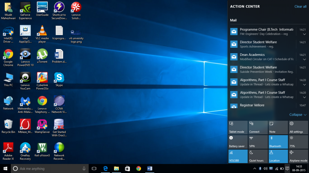
Task View Button
The new Task View button on the taskbar introduces the idea of moving between windows to the vast majority of Windows users who’ve never tried Alt Tab. We can hide or unhide this by right clicking on the taskbar and selecting the appropriate option.
Snap Assist
SnapAssist does more than the ‘two desktop apps getting half the desktop’ layout that you get in Windows 8. If one has one narrow window, the second window can take up all the rest of the space, or one can snap four apps, one in each corner. Windows will even show thumbnails of open windows to help the user to pick the one ,user wants to snap without rearranging everything.
Cortana
Cortana i.e. a personal assistant is a new feature added to Windows 10. One can ask, interact with Cortana and Cortana will reply with a suitable answer. Cortana is built into Spartan and attempts to predict and answer queries.(e.g. restaurant information) straight from browser.
What is the time dear Cortana??
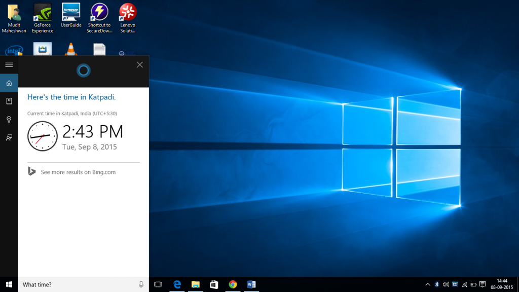
Microsoft Edge Browser
Microsoft Edge is the new default browser of Windows 10. It uses a clean GUI. It provides a hub facility to keep all the stuff in one place. It has a much better performance compared to Internet Explorer. Get the news feed from MSN. View the sites visited by the user mostly in the section Top sites.It’s been built with ‘interoperability’ in mind, according to Microsoft. Features include a reading mode and the ability to annotate, either with a keyboard, pen or a finger. There’s also integration with Cortana to provide additional information– for example, when the user is on a web page for a restaurant, Cortana will make a booking and display information such as opening times.
XBOX App And Streaming
There’s good news for gamers as not only with the Xbox One get Windows 10 (including Universal apps – see below), Microsoft has introduced some sweet new features. Windows 10 comes with the Xbox app which has features like the ability to control the Xbox One and a DVR capture for any Windows games.
Furthermore, user will be able to play multiplayer games cross-platform between Xbox One and PC. As if that wasn’t enough, Windows 10 will support the ability to stream games from the Xbox Box – although we don’t have details on the technical requirements for this yet. Oh and there’s support for DirectX 12.

Universal Apps
The news of Universal apps is good news for anyone using more than one Windows device. A bundle of apps including Photos, Videos, Music,Maps, People & Messaging and Mail & Calendar (and presumably more in the future) will look and feel the same across different devices and screen sizes. The data will also be saved and sync automatically via OneDrive.
Improvements to Windows Explorer
A new Home location is the new default view in Windows Explorer. There’s also a Share button on the Windows Explorer taskbar
Pros :
Cost free upgradation valid till 1 year. The upgrade is valid for lifetime.
New refreshed Web Browser
Universal app approach by Microsoft
Full XBOX Support
Easy,handy,useful,compact, complete, beautiful GUI, user friendly, light, awesome support to tablets, desktop are the major pros.
Cons:
Bluetooth driver may not work correctly. i.e. File can’t be received from other devices.
Digital Dolby sound driver may not work in the beginning.
Mail app may give syncing error problems which are yet to be resolved.
Battery performance has reduced probably due to the added features.
Control Panel
The Control Panel in Microsoft Windows enables a user to change various computer hardware and software features. Settings for the mouse, display, sound, network, and keyboard represent a few examples of what may be modified in the Control Panel. Below are examples of how the Control Panel appeared in Windows.
Sections of the Windows Control Panel
There are eight main areas on the Control Panel, containing different tools designed to optimize your computer.
System and Security - A section to check your computer's status, backup and restore, and others.
Network and Internet - View network status.
Hardware and Sound - View which devices are on your computer and add devices.
Programs - Uninstall programs.
User Accounts - Change user accessibility.
Appearance and Personalization - Change desktop options, like fonts and screen readers.
Clock and Region - Change date and time.
Ease of access - Optimize your display settings.
The evolution of the Windows Control Panel

Microsoft Windows 7 Control Panel

Microsoft Windows XP Control Panel

Microsoft Windows 98 Control Panel
My Computer
My Computer is a Microsoft Windows feature first found in Windows 95 and included with all later versions that allows you to explore and manage the contents of your computer drives. The image shows examples of the My Computer icon in Microsoft Windows XP, Vista and Windows 7, and the "This PC" icon in Windows 8 and in Windows 10. Although the name has changed, "This PC" still has the same functionality as "My Computer."
How to open My Computer
In all Windows versions, you can use the keyboard to open My Computer without using the mouse. Pressing the shortcut keys Windows key+E opens My Computer (Explorer). Your computer's drives and any installed devices are listed under the "This PC" section on the left.
or
Get to the Windows desktop and open Start menu, or navigate to the Start Screen if you are using Windows 8.
In earlier versions of Windows, after clicking Start, select My Computer. Or, on the desktop, double-click the My Computer icon. In Windows Vista and Windows 7, select Computer from the Start menu. In Windows 8 and Windows 10, select This PC from the Window's File Explorer.
Missing My Computer, My Network Places, or My Documents icon.
The following images show examples of the My Computer option in both new and old versions of Windows.
Windows XP
Note
In Windows Vista and Windows 7, My Computer is called "Computer" and is accessed through the Start menu, as shown below.

Windows 7
Note
In Windows 8, Windows 8.1, and Windows 10, My Computer is called "This PC" and is accessed through the Start menu.

How to use My Computer
Once My Computer (This PC) is open, you will see all available drives on your computer. The primary location of all your files is the Local Disk (C:), which is the default hard drive that stores all files. Double-click this drive icon to open it and view its contents.
Finding files in My Computer
Most files you create or will want to find are located in your My Documents folder. If you are having trouble finding where a file is stored, you can also use the Windows find feature.
How to find a file on a computer.
Finding My Computer on a Mac
On a macOS system, there is a similar section to My Computer called the Computer Folder. To access the Computer Folder, press Shift+Command+C.
Adjust system settings with My Computer
To manage or view your computer settings, right-click the My Computer icon and then click Properties. Performing these steps opens your System Properties (the same window accessible through the Control Panel).
Windows Explorer
Windows Explorer is the file manager used by Windows 95 and later versions. It allows users to manage files, folders and network connections, as well as search for files and related components. Windows Explorer has also grown to support new features unrelated to file management such as playing audio and videos and launching programs, etc. The desktop and the taskbar also form part of Windows Explorer. The look, feel and functionalities of Windows Explorer have been enhanced with each version of Windows.
Starting with Windows 8.0, Windows Explorer has been called File Explorer.
Log Off
To Log off/Shut down the computer:
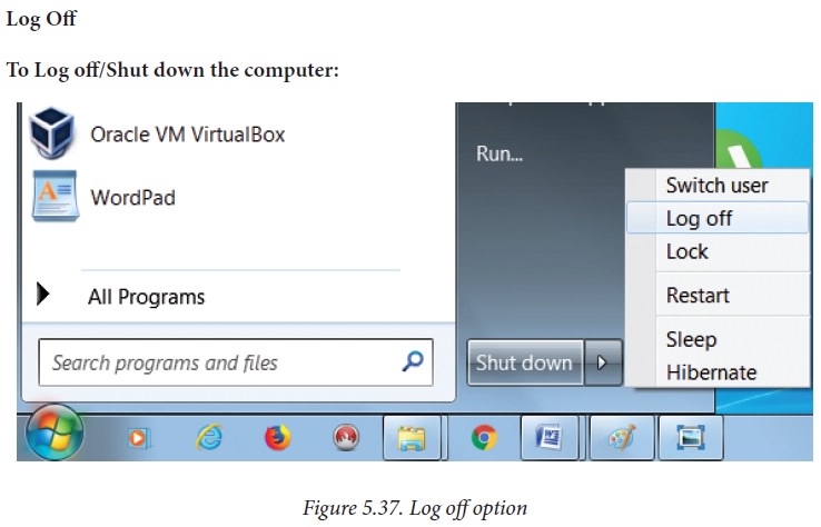
· Click start -> log off (click the arrow next to Shut down) or Start -> Shutdown . (Figure 5.37.)
· If you have any open programs, then you will be asked to close them or windows will Force shut down, you will lose any un-saved information if you do this.
· Switch User: Switch to another user account on the computer without closing your open programs and Windows processes.
· Log Off: Switch to another user account on the computer after closing all your open programs and Windows processes.
· Lock: Lock the computer while you're away from it.
· Restart: Reboot the computer. (This option is often required as part of installing new software or Windows update.)
· Sleep: Puts the computer into a low-power mode that retains all running programs and open Windows in computer memory for a super-quick restart.
· Hibernate (found only on laptop computers): Puts the computer into a low-power mode after saving all running programs and open Windows on the machine's hard drive for a quick restart.


Comments
Post a Comment